Follow @solverworld Tweet this

“All about X, part 1” is really a fancy way of saying a little bit about X.

How do you eat an elephant?
One bite at a time ¹

So let’s eat stochastic difference equations one bite at a time. Let’s consider a first-order linear equation driven by a Gaussian random variable.

\begin{align}
x_{n+1}&=ax_n+w_n \\
w_n &\sim N(0, \sigma^2) \\
|a| & < 1. \\
\end{align}

Let’s dissect this one bit at a time. \(x_n \) is our system’s state, or value, at time \(n \). Our time variable \(n \) takes on integer values, -2, -1, 0, 1, 2, and so on. \(w_n\) is our noise term, and it is a normally distributed Gaussian variable with mean 0 and standard deviation \(\sigma\) at each time \(n\). The values at different times are uncorrelated. We require \(|a|<1\) so that our equation is stable, or does not blow up.
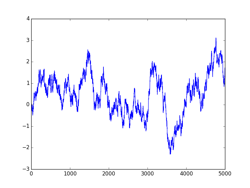
What does this series look like? Here is a sample run of 5000 steps for a=0.9967 and \(\sigma=\)0.082. The significance of these numbers will be revealed later.

Let’s derive some basic properties of our stochastic series \(x_n\). Recall that \(E()\) is the expectation operator, meaning it computes the expected value of its random variable argument.

\(\newcommand{\Var}{\mathrm{Var}}\)
\(\newcommand{\Cov}{\mathrm{Cov}}\)
\(\newcommand{\Expect}{{\rm I\kern-.3em E}}\)

What is the average (expected) value of \(x_n\)? Since our process is stationary, that is, a is fixed, and \(w_n\) does not varying it’s statistics over time, \(\Expect(x_n)\) is constant, let’s call it \(\Expect(x)\). Then

\begin{align}
\Expect(x_{n+1})&=a\Expect(x_n)+\Expect(w_n) \\
\Expect(x)(1-a)&=\Expect(w_n) \\
\Expect(x)&=0
\end{align}
where we used \(E(w_n)=0\) for the final step.

What about the variance of x?
\begin{align}
\Var(x_{n+1})&=a^2\Var(x_n)+\Var(w_n) \\
\Var(x)(1-a^2)&=\sigma^2 \\
\Var(x)&=\frac{\sigma^2}{1-a^2}
\end{align}
\begin{align}
\Cov(x_{n+1},x_n)&=\Expect[(x_{n+1}-\Expect(x_{n+1}))(x_{n}-\Expect(x_{n}))]\\
&=\Expect[x_{n+1}x_{n}]\\
&=\Expect[(ax_n+w_n)x_n]\\
&=\Expect[ax_n^2]\\
&=\frac{a\sigma^2}{1-a^2}
\end{align}

Let’s look at the increments:
\begin{align}
\Delta x_{n+1}&=x_{n+1}-x_n\\
&=(a-1)x_n+w_n\\
\Var(\Delta x)&=(a-1)^2\Var(x)+\sigma^2\\
\Var(\Delta x)&=\sigma^2[\frac{(1-a)^2}{1-a^2}+1]\\
&=\sigma^2\frac{2}{1+a}.
\end{align}
Note If a is close to 1, then the variance of the increments is close to \(\sigma^2\).

Now, let’s get a little more involved and compute the variance over k steps. From some basic system theory (or inspection):
\begin{align}
x_k=x_0 a^k + \sum_{s=0}^{k-1}a^{k-s-1}w_s
\end{align}
To make sure we have the right limits, let’s check for k=1:
\[
x_1=a x_0 + w_0
\]
That looks right, let’s continue on.
\begin{align}
\Var(x_k-x_0)=(a^k-1)^2\Var(x)+\sigma^2\sum_{s=0}^{k-1}(a^{k-s-1})^2
\end{align}
Now, using the Sum of a Geometric Series, we have
\begin{align}
\Var(x_k-x_0)&=\frac{(a^k-1)^2}{1-a^2}\sigma^2 + \frac{1-a^{2k}}{1-a^2}\\
&=\sigma^2 [ \frac{(a^k-1)^2 + 1 – a^{2k}}{1-a^2}\\
&=2 \sigma^2 \frac{1-a^k}{1-a^2}.
\end{align}
Checking when \(k=1\) and we see it matches our earlier result.

In Part 2 we will look more closely at some simulations and trading results on these series.

Follow @solverworld Tweet this

What is the sum of the following geometric series?
\[
\sum_{i=0}^{k}a^i=1+a+a^2+…+a^k
\]
We will frequently need a simple formula for this finite series. It is called a geometric series because each term is related by a multiple to the previous one. If each term was related by a fixed difference, it would be called an arithmetic series; but that’s for another day.
Let us define the sum as \(S\). Then writing the equation for \(S\) and \(aS\) with some clever alignment:

\begin{array}{rrrccc}
S=&1&+a&+a^2&+…&+a^k \\
aS=&&a&+a^2&+…&+a^k&+a^{k+1}
\end{array}
Subtract the equations
\[
S(1-a)=1-a^{k+1}
\]
or
\begin{align}
S=
\begin{cases}
\frac{1-a^{k+1}}{1-a} &a \neq 1 \\
k+1 &\text{otherwise}
\end{cases}
\end{align}
where we have to be careful to divide by \(1-a\) only if \(a\neq 1\), and the answer for \(a=1\) is determined by inspection.
Q.E.D.

Follow @solverworld Tweet this

You may have seen the following equation:
\begin{align}
\lim_{n \rightarrow \infty} \left( 1 +\frac{1}{n} \right)^n = \mathrm{e}.
\end{align}

which expresses the fundamental constant e as a limit. Wondering how that can be proven?

Consider this graph:

One key fact we will use is

\begin{align}
\int_1^{x} \, \frac{1}{t} \mathrm{d}t = \ln x
\end{align}

Looking at the graph, you can see that the area under the \(\frac{1}{t}\) curve on the interval \((1,1+\frac{1}{n})\) is bounded by

\begin{align}
\frac{1}{n}\left( \frac{1}{1+\frac{1}{n}} \right) \leq \int_1^{1+\frac{1}{n}} \, \frac{1}{t} \mathrm{d}t \leq \frac{1}{n} \left( 1 \right)
\end{align}

Using the definition of \(\ln x\) above, we have

\begin{align}
\frac{1}{1+n} \leq \ln \left( 1+\frac{1}{n} \right) \leq \frac{1}{n}
\end{align}

Raising \(\mathrm{e}\) to the power of each term,

\begin{align}
\mathrm{e}^{(\frac{1}{1+n})} \leq 1+\frac{1}{n} \leq \mathrm{e}^{(\frac{1}{n})}
\end{align}

Raising each term to power \(n\),
\begin{align}
\mathrm{e}^{(\frac{n}{1+n})} \leq \left( 1+\frac{1}{n} \right)^n \leq \mathrm{e}
\end{align}

As n approaches infinity, the left hand term approaches \(\mathrm{e}\), therefore
\begin{align}
\lim_{n \rightarrow \infty} \left( 1 +\frac{1}{n} \right)^n = \mathrm{e}.
\end{align}

QED.