Installing BOINC on Multi GPU Computer

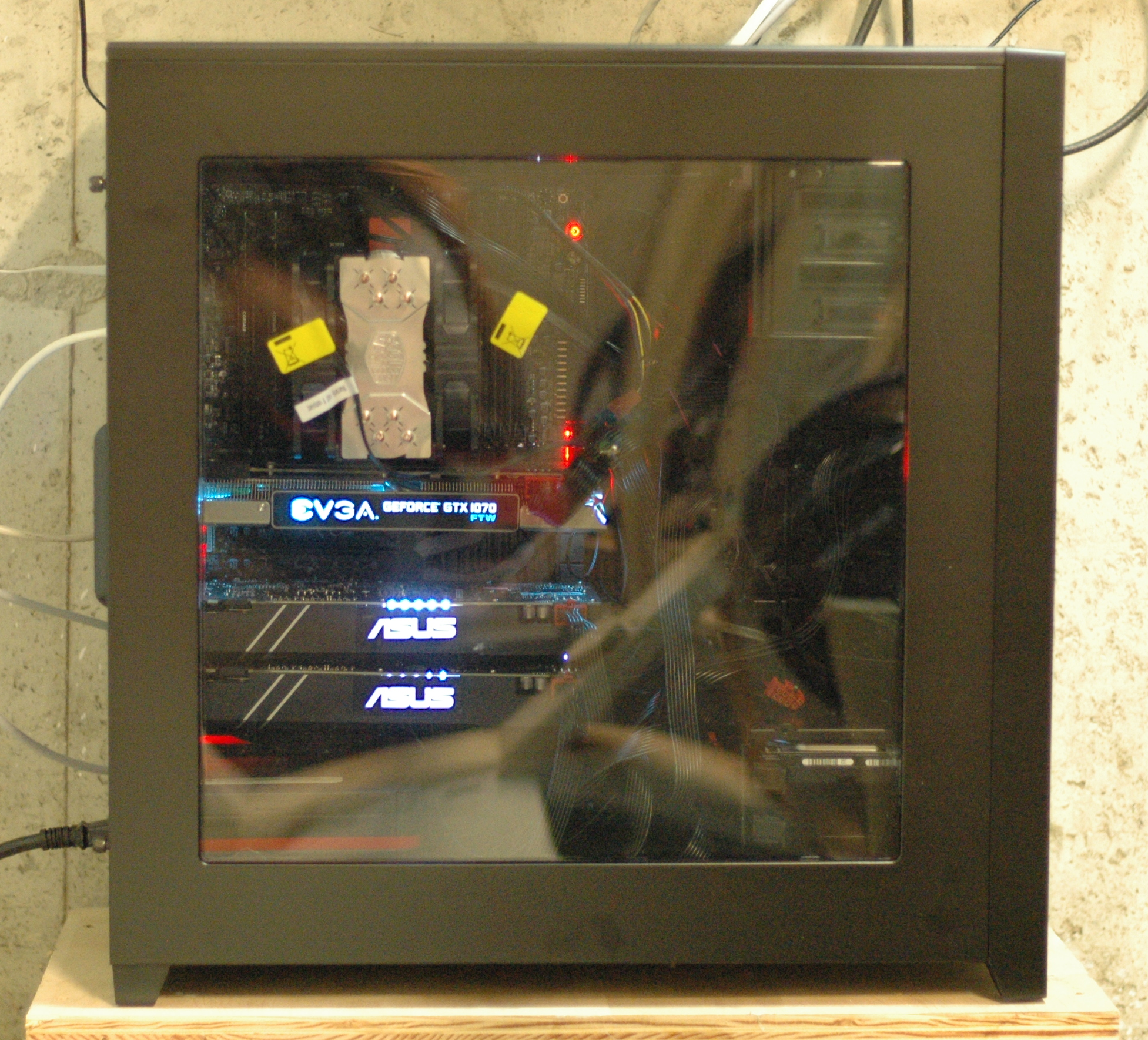
Computer GPUs lit up

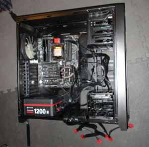
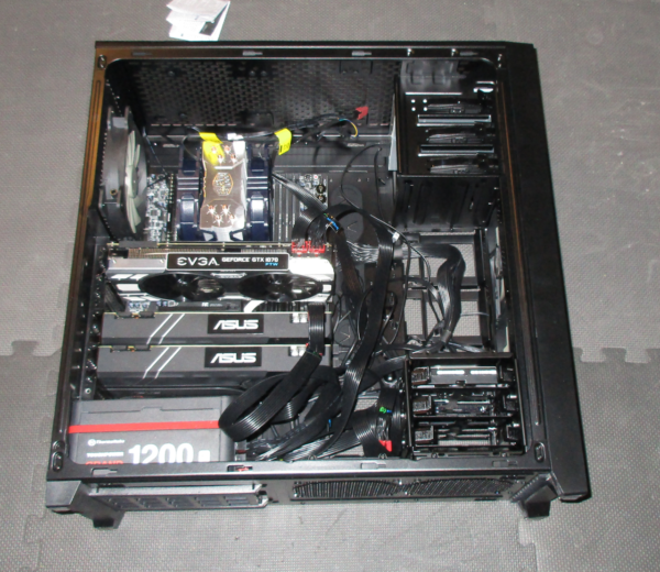
Already built a multi-GPU computer?  No?  See How to Build a Multi-GPU Computer here.

OK, we have our multiple GPU system wired up and it seems to boot OK into the BIOS.  The BIOS shows our 3 GPUs installed in the proper slots and we like the speeds (Gen 3) of PCIe that are chosen.

Let’s install Linux.  I choose Debian – I am familiar with it, and more importantly, I got it to work with BOINC.  Here is that procedure:

  1. Create a netinst DVD or CD for Debian Stretch.  I found that the latest stable version (Jessie) did not have the correct packages to get BOINC running.  I used RC2, but RC3 is available now, and should work as well.  Ddownload the .iso file you need (probably the amd64 package) to your computer, then use an ISO writing program to write that to a DVD/CD.  On a Windows machine, I used ImgBurn, but you can use any program you like.
  2. Boot the multi-GPU computer with this DVD.   If it does not boot from the DVD drive, you will need to go into the BIOS and set up the boot order so that the DVD is first or at least tried after the HDD fails.
  3. Follow the prompts to install Debian.  There are plenty of guides on the Internet to help you, but it is pretty straightforward.  You can take defaults for just about everything.  I did NOT install the desktop environment because I only plan on ssh’ing into the computer and did not want to have X software installed/running.  Do choose ssh server and standard system utilities.  NOTE: you will need an Internet connection, preferably hardwired, to install Debian, so plug in an Ethernet cable to your Internet connection before you start.
  4. Install sudo so you can become root as needed – first log in as root, then
    apt-get install sudo
    usermod -aG sudo <your-user-name>
  5. Add contrib and non-free to your /etc/apt/sources.lst file as some of the nvidia driver files are in those categories.  You should have a line in the sources.lst file that looks like:
    deb http://ftp.us.debian.org/debian/ stretch main non-free contrib
  6. Update your database:
    sudo apt-get update
  7. To be able to ssh into this machine without a password, add your public key which you have copied to this machine already, to the list of authorized keys.  Note that you could transfer the key with a USB key if you don’t want to copy over the network:
    sudo mount /dev/sdb1 /media/usb    # your devices may differ
    cat /media/usb/id_rsa.pub >> ~/.ssh/authorized_keys
  8. Now install the BOINC software and related drivers.  You might want to install them sequentially to make debugging simpler in case something goes wrong.  I got nvidia-driver version 375.26-2.
    sudo apt-get install nvidia-driver boinc-client-opencl boinc-client-nvidia-cuda boinc
  9. Make sure the BOINC client autostarts on boot up – check your /etc/init.d/ directory for a boinc-client script.  Now, a small adjustment is necessary to make sure the GPUs are detected at startup – there is a race condition with drivers, so edit the boinc-client script (as root) and add a sleep 2.0 line so that the start() function in the file looks like:
    start()
    {
     log_begin_msg "Starting $DESC: $NAME me"
     sleep 2.0    #<== ADD THIS LINE
     if is_running; then
       log_progress_msg "already running"
     else
       if
  10. Now, you should be able to reboot the computer and see something like the following from ps -ef:
    #ps -ef |grep boinc
    dan      614 24444 0 17:17 pts/0 00:00:00 grep boinc
    boinc    623 1     0 Mar30 ?     00:00:00 /bin/sh -c /usr/bin/boinc --dir /var/lib/boinc-client >/var/log/boinc.log 2>/var/log/boincerr.log
    boinc    641 623   0 Mar30 ?     00:30:05 /usr/bin/boinc --dir /var/lib/boinc-client
    

    If you can’t see boinc, running you will need to do some debugging.  Check out /var/log/boinc.log and you can see the startup messages.  If everything is going well, you will see the GPUs being detected and indicating how many are usable (hopefully the number you installed, in this case 3).  Some debug steps are:  (i) try nvidia-smi to see if the Nvidia drivers can see your GPUs, and (ii) set the BOINC logging flags – possibly <coproc_debug> in BOINC Configuration.

  11. A couple more things and we are almost done.  To enable remote management of the BOINC server software, add/edit the following files in /var/lib/boinc_client:
    echo <remote-access-password> > gui_rpc_auth.cfg
    echo <your-remote-access-IP-address> > remote_hosts.cfg
  12. Now you should be able to connect to the server through the boincmgr program, using the password you set above.  You can install BOINC on a windows or linux machine fairly easily, which will give you access to the manager program.  Of course, if you want to keep your GPU machine in a place where you can access it via keyboard and monitor, you could just run the boincmgr locally.  Note that it will not run unless you install a Desktop environment, since it needs X-client running.
  13. From the manager program, you can select a project from the available ones on BOINC such as SETI, primegrid, etc.  You will have to provided credentials to get you started, which you get by creating an account on the appropriate projects website (e.g. primegrid.com).  For Primegrid, you can control which tasks your computer works on through configuring things on the primegrid website.  Note that only certain tasks can take advantage of the Nvidia-cuda GPUs, so make sure you select at least 1 subproject that does that.  Other tasks can be run on the CPU directly, but make sure not to fully load your CPU with tasks, as that will tend to slow down the servicing of the GPUs.
  14. If your computer will have any exposure to the outside world (including your home WiFi), you should be careful to secure it properly.  At a minimum, you will want to disable root logins, all unnecessary processes and open ports.
  15. Join the SolverWorld team on PrimeGrid and add your computing power to the team.  I will announce your contributions (if you want) on separate page in the future.
  16. Happy computing!

Building a Multiple GPU Computer for Grid Computing

Computer with three GPUs running

Introduction

Want to search for evidence of extraterrestrial life? Want to find your very own prime number?  One way to do this is to join a grid computing project.  The Berkeley Open Infrastructure for Network Computing (BOINC) is a framework for people creating grid computing projects.

A video from Matt Parker and Numberphile, 383 is cool, sparked huge interest in the Primegrid project on BOINC.  You can join BOINC and Primegrid with just about any computer (I will give some instructions in a later post), but for doing real supercomputing, you will want to use a GPU (Graphics Processing Unit).  GPUs have traditionally have used for gaming purposes, but as scientists realized the computing power inherent in the GPU, uses outside gaming started to proliferate.  A single GPU unit can perform calculations 50-200 times faster than a single CPU.

This post will discuss how to build a computer with 3 powerful GPUs that is still climbing up the contributor’s rank list at Primegrid – I hope to make it to the top 3.

To incorporate multiple GPUs in a single case, there are a number of things to worry about that you don’t worry about in a basic CPU and motherboard build:

  • CPU – CPUs have a limited number of PCIe “lanes” available that have to be split up amount all the GPUs.  The latest generation (7th) of Intel processors, such as the i7-7700, have 16 lanes of PCIe, so they could do one GPU at x8 and two at x4.  We want to go faster, so we picked an i7-6850K, which, while an older generation and lower clock speed, has 40 lanes of PCIe, and thus, we will be able do 3 GPUs at x16, x16, and x8.
  • Motherboard – you need to be able to fit all the GPUs into PCIe slots.  GPUs are typically double wide (take up 2 slot spaces).  You want enough PCIe lanes to keep each GPU humming at full capacity.  If you are going to spend all those dollars on top-end GPUs, you want to fully utilize them.  The exact number of lanes you need will depend on the project you are working on.  For this computer build, I decided I wanted to keep as many GPUs running at x16 (full bandwidth) as I could – experiments later could help determine if they are all needed.  Of course, the motherboard must be slot compatible with the CPU you choose.  For the 6850K we will need a socket LGA 2011 motherboard.
  • Case – the case needs to hold the motherboard you chose (obviously), and have lots of fans to dissipate all the heat that will be generated.  Also, it will be nice to have extra of room to maneuver as we fit in all the cards, fans, and power supplies inside.
  • Power supply – You need enough power for all the parts you have selected.  Each GPU will use up to about 200W (check the specs).  Also, since we will be using lots of power and we want to keep our operating costs down, more efficiency will be worthwhile.  Using a smaller fraction of a power supply’s capacity (maybe 50%) will generally improve efficiency also.  Also consider if you will be adding more components later, as taking apart the machine to upgrade the power supply later might not be convenient.
  • GPUs – the muscles of the machine.  Nvidia-based GPUs are popular.  The most powerful one currently is the GTX1080, but since i already had a GTX1070, I decided to go with them by adding 2 more.  You can check with your particular project to see what the cost/performance tradeoff is for various GPUs.  The ASUS ones have a design that sends the airflow out the back of the case, where the IO connectors are, which seems better in a multi-GPU setup than the EVGA design that blows hot air on the GPU next to it.

The Machine

Before we get into building the computer, here are the parts we selected:

  • Case – Corsair 750D Full-tower.  Anyone used to wimpy mid-tower cases will be totally impressed with this monster.
  • CPU – i7-6850K 40 lane processor.  Uses socket LGA-2011
  • Motherboard – EVGA X99 FTW.  This is compatible with the 6850K, and can hold 128GB of RAM
  • RAM – 16GB of 2400 MHz DDR4.  We don’t need huge amounts of memory for the BOINC projects we are running, but your needs might vary.
  • CPU cooler – Hyper 212X Turbo
  • Power supply – Thermaltake Grand Platinum 1200W.  Probably overkill, but better safe than sorry.
  • Hard drive – I just used a 1 TB HDD lying around.  GPU computing projects generally don’t need speedy disks, but if you wanted to boot faster, you could replace with a SSD (solid state drive).
  • DVD drive – not completely necessary, but makes it easier to boot up and install your operating system
  • Monitor – you will want a monitor to install the OS and configure it, even though you do not need it once you are chugging away looking for aliens.  You will also need it to configure the BIOS, and also keep in mind that the motherboard used here does not have built in graphics, so a VGA monitor has nowhere to plug in. You will need an inexpensive HDMI or DVI monitor.  And keyboard for setup.
  • GPUs – I used one EVGA GTX1070 and two ASUS GTX1070 Turbo VR Ready editions.  This ASUS edition has the fans that exhaust out the back.
  • OS – I choose Debian linux.  It’s free, and below I will show how to install it to get the GPUs working on BOINC.

Building It

Case with power supply before other stuff.  The order you assemble this computer can reduce the hassles, so here is what I found worked for me.

This picture shows the computer with the motherboard and power supply installed, before the CPU cooler and GPUs go in.


  1. Remove second HDD cage closest to power supply area, otherwise 3rd GPU won’t fit
  2. Put in HDD and DVD and wire up
  3. Install power supply.  This heavy item should go in before delicate components to come.
  4. Insert CPU
  5. Insert memory (do this before CPU cooler because it sits below heatsink)
  6. CPU cooler
  7. Wire up the fans (do the before GPUs).  One of the front fans wires was tucked under the HDD cage and I overlooked it the first time.
  8. Insert GPUs
  9. Add the power supply connectors to the motherboard and to the GPUs.  Make sure you follow your motherboard and GPU instructions.  You can also add a extra PCIe bus power connector to the motherboard, which seems like a good idea given all the PCIe boards we just installed.

Here is what the finished install looks like.  You can see that we have room for one more GPU, if we want to go all out!

The CPU cooler fans are oriented to blow air towards the back of the case.  This is a must since the front fans and back fan are oriented the same way.  There is a very small, yet positive, clearance between the CPU cooler and the EVGA GPU.

Once everything is wired up and double checked, hook up a DVI/HDMI monitor and keyboard and fire it up.

You should adjust any BIOS settings you need before installing the OS.
Next post:
installing BOINC on multi-GPU computer


Relevant items at Amazon: (If you can’t see them, turn off your ad blocker)

Buy NVIDIA GTX 1080 at Amazon


Trading Stochastic Difference Equations

If you haven’t read Part 1, do that first.
\(\newcommand{\Var}{\mathrm{Var}}\)
\(\newcommand{\Cov}{\mathrm{Cov}}\)
\(\newcommand{\Expect}{{\rm I\kern-.3em E}}\)
\(\newcommand{\me}{\mathrm{e}}\)
For a quick review, recall that our system looks like:
\begin{align}
x_{n+1}&=ax_n+w_n \\
w_n &\sim N(0, \sigma^2) \\
|a| & < 1. \\
\end{align}
Next, let’s define a time constant, \(\tau\), that gives us an idea of how the noise term, \(w_n\), is filtered. Time constants are generally the time it takes to reach \(1/\me\) of a steady-state value, so:
\begin{align}
&\frac{1}{\me}=a^\tau \\
&-1=\tau \ln a\\
&\tau=\frac{-1}{\ln a}\\
\text{or}\\
&a=\me^{-1/ \tau}
\end{align}

Now, our goal is to understand how we could trade (profitably) such a stochastic system. What does this mean? We might want to try something like, “buy low, sell high.” Like
\begin{align}
x_n \leq T_1&\Rightarrow \text{buy}\\
x_n \geq T_2&\Rightarrow \text{sell}
\end{align}
Our profit on each round-trip trade would be \(T_2-T_1\). Hopefully, we choose \(T_2 > T_1\).

Thresholds

Since our system is linear, scaling the input (\(w_n\)), scales the output. Thus, if we set thresholds as a multiple of \(\sigma\) we do not have to explore different noise powers. Put another way, if we fix, say, \(\Var(x)\equiv 1\), then we can experiment with different thresholds, and the results will hold for those thresholds as a multiple of \(\Var(x)\).

Time Durations

Similarly, if we are counting events (trades) over time, we want to be able to scale everything to a useful value.
Consider (from Part 1):

\begin{align}
\Var(x_k-x_0)&=2 \sigma^2 \frac{1-a^k}{1-a^2} \\
&=2\Var(x)(1-a^k)\\
&=2\Var(x)(1-\me^{-k/\tau})
\end{align}
We can see that the variance of increments depends on the number of time constants that we go out. So, if we count trades per time constant interval, we will have standardized our results. Note: The astute reader should note that this is not a proof (not even close), but we will leave that for later. This is more of a “seems plausible.”

Some Simulations

Let’s perform a few tests to get started. We will pick an \(a\) corresponding to \(\tau\) of [300, 600, 1200] time steps (think seconds), and then fix \(\sigma\) to make \(\Var(x)\equiv 1\). Then we will perform Monte Carlo simulations over enough time steps to get statistically significant results.

Here are the results.
round trip trades vs. threshold

There are 2 types of trading algorithms simulated here:

  • -t/+t: buy when x<-t and sell when x>+t, count action as 0.5 trades
  • -2t/0/+2t: buy when x<-2t and sell when x>0; plus sell when x>2t and buy when x<0

Each of these has a 2t profit per round trip trade, but the second option occurs more often for smaller thresholds.  For larger thresholds, the rapid Gaussian falloff causes there to be fewer trades.

Note you can see that the three different time constant (TC) values have lines very close to each other, justifying our supposition that events per TC are the relevant experimental parameter.  This means we can do our simulations for a single TC, rather than a whole series.

If we multiple the number of trades by the profit per trade, we get the following result.  Of course, this ignores commissions, which would drag down the profits more on the lower thresholds (more trades).

total profit vs. threshold

The simulations used 200,000 time steps, and the following parameters.

time constant (steps)astd dev of wstd dev of x
300.99667.0821.031
600.99833.0581.029
1200.99917.0411.005

All About Stochastic Difference Equations, Part 1

“All about X, part 1” is really a fancy way of saying a little bit about X.

How do you eat an elephant?
One bite at a time 1

So let’s eat stochastic difference equations one bite at a time. Let’s consider a first-order linear equation driven by a Gaussian random variable.

\begin{align}
x_{n+1}&=ax_n+w_n \\
w_n &\sim N(0, \sigma^2) \\
|a| & < 1. \\
\end{align}

Let’s dissect this one bit at a time. \(x_n \) is our system’s state, or value, at time \(n \). Our time variable \(n \) takes on integer values, -2, -1, 0, 1, 2, and so on. \(w_n\) is our noise term, and it is a normally distributed Gaussian variable with mean 0 and standard deviation \(\sigma\) at each time \(n\). The values at different times are uncorrelated. We require \(|a|<1\) so that our equation is stable, or does not blow up.
What does this series look like? Here is a sample run of 5000 steps for a=0.9967 and \(\sigma=\)0.082. The significance of these numbers will be revealed later.

sde_a0-9967_w0-082

Let’s derive some basic properties of our stochastic series \(x_n\). Recall that \(E()\) is the expectation operator, meaning it computes the expected value of its random variable argument.

\(\newcommand{\Var}{\mathrm{Var}}\)
\(\newcommand{\Cov}{\mathrm{Cov}}\)
\(\newcommand{\Expect}{{\rm I\kern-.3em E}}\)

What is the average (expected) value of \(x_n\)? Since our process is stationary, that is, a is fixed, and \(w_n\) does not varying it’s statistics over time, \(\Expect(x_n)\) is constant, let’s call it \(\Expect(x)\). Then

\begin{align}
\Expect(x_{n+1})&=a\Expect(x_n)+\Expect(w_n) \\
\Expect(x)(1-a)&=\Expect(w_n) \\
\Expect(x)&=0
\end{align}
where we used \(E(w_n)=0\) for the final step.

What about the variance of x?
\begin{align}
\Var(x_{n+1})&=a^2\Var(x_n)+\Var(w_n) \\
\Var(x)(1-a^2)&=\sigma^2 \\
\Var(x)&=\frac{\sigma^2}{1-a^2}
\end{align}
\begin{align}
\Cov(x_{n+1},x_n)&=\Expect[(x_{n+1}-\Expect(x_{n+1}))(x_{n}-\Expect(x_{n}))]\\
&=\Expect[x_{n+1}x_{n}]\\
&=\Expect[(ax_n+w_n)x_n]\\
&=\Expect[ax_n^2]\\
&=\frac{a\sigma^2}{1-a^2}
\end{align}

Let’s look at the increments:
\begin{align}
\Delta x_{n+1}&=x_{n+1}-x_n\\
&=(a-1)x_n+w_n\\
\Var(\Delta x)&=(a-1)^2\Var(x)+\sigma^2\\
\Var(\Delta x)&=\sigma^2[\frac{(1-a)^2}{1-a^2}+1]\\
&=\sigma^2\frac{2}{1+a}.
\end{align}
Note If a is close to 1, then the variance of the increments is close to \(\sigma^2\).

Now, let’s get a little more involved and compute the variance over k steps. From some basic system theory (or inspection):
\begin{align}
x_k=x_0 a^k + \sum_{s=0}^{k-1}a^{k-s-1}w_s
\end{align}
To make sure we have the right limits, let’s check for k=1:
\[
x_1=a x_0 + w_0
\]
That looks right, let’s continue on.
\begin{align}
\Var(x_k-x_0)=(a^k-1)^2\Var(x)+\sigma^2\sum_{s=0}^{k-1}(a^{k-s-1})^2
\end{align}
Now, using the Sum of a Geometric Series, we have
\begin{align}
\Var(x_k-x_0)&=\frac{(a^k-1)^2}{1-a^2}\sigma^2 + \frac{1-a^{2k}}{1-a^2}\\
&=\sigma^2 [ \frac{(a^k-1)^2 + 1 – a^{2k}}{1-a^2}\\
&=2 \sigma^2 \frac{1-a^k}{1-a^2}.
\end{align}
Checking when \(k=1\) and we see it matches our earlier result.

In Part 2 we will look more closely at some simulations and trading results on these series.

Notes:

  1. Generally credited to General Creighton Williams Abrams, Jr., Chief of Staff of United States Army 1972-1974, but an earlier reference to the concept is Frank Cody, Detroit’s Superintendent of Schools in 1921 link