Follow @solverworld Tweet this

If you haven’t read Part 1, do that first.
\(\newcommand{\Var}{\mathrm{Var}}\)
\(\newcommand{\Cov}{\mathrm{Cov}}\)
\(\newcommand{\Expect}{{\rm I\kern-.3em E}}\)
\(\newcommand{\me}{\mathrm{e}}\)
For a quick review, recall that our system looks like:
\begin{align}
x_{n+1}&=ax_n+w_n \\
w_n &\sim N(0, \sigma^2) \\
|a| & < 1. \\
\end{align}
Next, let’s define a time constant, \(\tau\), that gives us an idea of how the noise term, \(w_n\), is filtered. Time constants are generally the time it takes to reach \(1/\me\) of a steady-state value, so:
\begin{align}
&\frac{1}{\me}=a^\tau \\
&-1=\tau \ln a\\
&\tau=\frac{-1}{\ln a}\\
\text{or}\\
&a=\me^{-1/ \tau}
\end{align}

Now, our goal is to understand how we could trade (profitably) such a stochastic system. What does this mean? We might want to try something like, “buy low, sell high.” Like
\begin{align}
x_n \leq T_1&\Rightarrow \text{buy}\\
x_n \geq T_2&\Rightarrow \text{sell}
\end{align}
Our profit on each round-trip trade would be \(T_2-T_1\). Hopefully, we choose \(T_2 > T_1\).

Thresholds

Since our system is linear, scaling the input (\(w_n\)), scales the output. Thus, if we set thresholds as a multiple of \(\sigma\) we do not have to explore different noise powers. Put another way, if we fix, say, \(\Var(x)\equiv 1\), then we can experiment with different thresholds, and the results will hold for those thresholds as a multiple of \(\Var(x)\).

Time Durations

Similarly, if we are counting events (trades) over time, we want to be able to scale everything to a useful value.
Consider (from Part 1):

\begin{align}
\Var(x_k-x_0)&=2 \sigma^2 \frac{1-a^k}{1-a^2} \\
&=2\Var(x)(1-a^k)\\
&=2\Var(x)(1-\me^{-k/\tau})
\end{align}
We can see that the variance of increments depends on the number of time constants that we go out. So, if we count trades per time constant interval, we will have standardized our results. Note: The astute reader should note that this is not a proof (not even close), but we will leave that for later. This is more of a “seems plausible.”

Some Simulations

Let’s perform a few tests to get started. We will pick an \(a\) corresponding to \(\tau\) of [300, 600, 1200] time steps (think seconds), and then fix \(\sigma\) to make \(\Var(x)\equiv 1\). Then we will perform Monte Carlo simulations over enough time steps to get statistically significant results.

Here are the results.

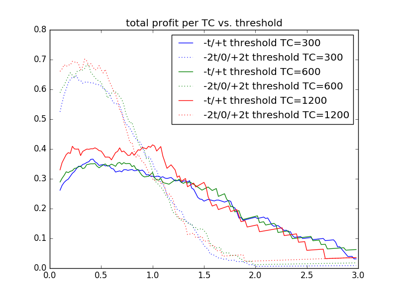
There are 2 types of trading algorithms simulated here:

• -t/+t: buy when x<-t and sell when x>+t, count action as 0.5 trades
• -2t/0/+2t: buy when x<-2t and sell when x>0; plus sell when x>2t and buy when x<0

Each of these has a 2t profit per round trip trade, but the second option occurs more often for smaller thresholds.  For larger thresholds, the rapid Gaussian falloff causes there to be fewer trades.

Note you can see that the three different time constant (TC) values have lines very close to each other, justifying our supposition that events per TC are the relevant experimental parameter.  This means we can do our simulations for a single TC, rather than a whole series.

If we multiple the number of trades by the profit per trade, we get the following result.  Of course, this ignores commissions, which would drag down the profits more on the lower thresholds (more trades).

The simulations used 200,000 time steps, and the following parameters.

time constant (steps)	a	std dev of w	std dev of x
300	.99667	.082	1.031
600	.99833	.058	1.029
1200	.99917	.041	1.005