

Follow @solverworld Tweet this
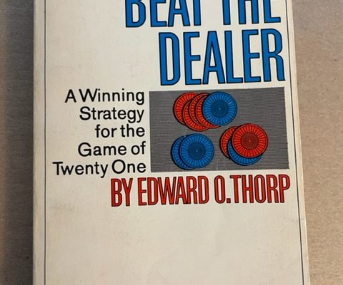
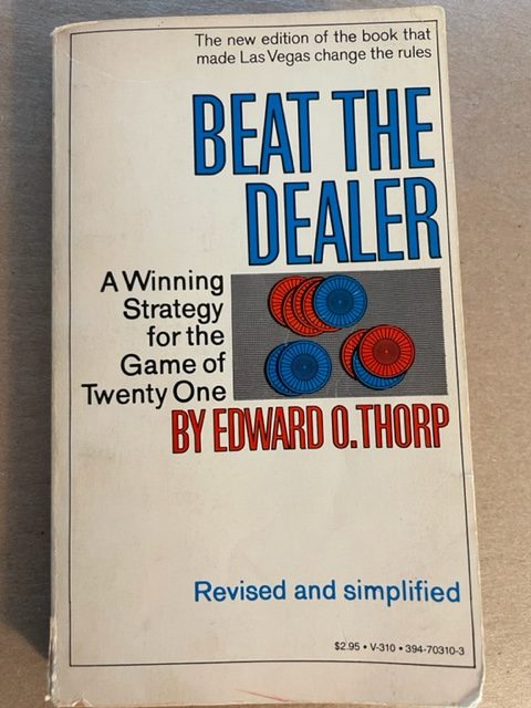
Beat the Dealer by Ed Thorp, published in 1962 (1966 rev. ed) laid out a winning strategy for playing Blackjack through card counting. While an earlier book Playing Blackjack to Win, by Roger Baldwin et al (1957) exists, and Thorp gives them due credit, Beat the Dealer is certainly the book that popularized the concept and sold over 1,000,000 copies.
When Professor Thorp did his calculations, computers were a little bit slower. I’d like to think he used the 1960’s version of a desktop computer: the Elliot Brothers 903 Elliot 903 description .
This machine had up to 64K of memory (core, not modern-day RAM), 18-bit words and a cycle time of 6 microseconds. The desktop computer I will use to recompute the basic Blackjack strategies has a 4 GHz clock rate, or 0.25 nanosecond cycle time (that’s about 24,000 times faster then the Elliot 903), not to mention (a) 64-bit words, (b) a million times more memory, (c) many more instructions than the handful the Elliot had, and (d) 8 cores running in parallel. Plus I can program in Python instead of FORTRAN or Assembly.
Unfortunately, Thorp did not use the Elliott. It was probably too slow. In his book’s acknowledgment, Thorp says he is grateful for the use of MIT’s IBM 704 computer. That’s this one:

What I would like to do is recalculate the Basic Strategy that Thorp outlined in his book. I will use a technique from Reinforcement Learning, by Sutton & Barlow. Rich Sutton is the father of reinforcement learning and I highly recommend his book as a well-written, clear and easy to understand introduction to the subject.
The technique we will implement is the one labeled “Monte Carlo ES (Exploring Starts)” in Chapter 5 of the second edition of Reinforcement Learning.
First, a little introduction to what we are doing. For the detailed description see Reinforcement Learning.
A strategy \(\pi\) is a function that maps the current state (what we can observe) into an action that we can take. There is a very simple (at least conceptually) way to compute how good any particular strategy is. We can simulate many games using this strategy and compute the value of the game. The value of the game is simply the average result that we can expect. In our game, we will say each game can result in a -1 (loss), +1 (win), or +1.5 (win with a Blackjack, or a natural 21). Of course, the other way to calculate the value of a strategy would be to calculate the probability of each outcome, and multiply those probabilities times the corresponding outcome – the sum of these would be the expected value of the outcome, what we call the “value” of the game. If I give you a strategy for Blackjack, which would be a table of what to do based on what you can see at each deal of the cards, and asked you to calculate the probability of winning, you can immediately see that this would be fairly complicated. For each deal, you would have to compute the probability of getting that deal, then the probability of getting each additional card (if you hit), and so on, each time following the strategy I gave you. On the other hand, the Monte Carlo method is much simpler. I just have the computer play lots of games using that strategy, and just add up the results. I am much less likely to make a mistake in computing things, because I am just counting, not computing probabilities. Of course, the answer I get is not exact, and I may have to do a lot of simulations to get reasonable precision, but why not let the computer do all the work, instead of me?
So we can see how to compute the value of a given strategy \(\pi\), but how would we go about finding the optimal strategy, usually written \(\pi^*\)? The idea is one of “policy improvement.” If we have a policy \(\pi\), can we improve it a little bit? The answer is yes. The idea is that when we calculated the value of a particular strategy, we computed a function \(q_\pi(s,a)\), which was the expected value (or return) when starting in state s and taking action a. The idea of policy improvement is that we make a slight change to \(\pi\) by making it greedy with respect to the \(q()\) function – that is
$$\begin{align}
\pi(s) = \arg \max_{a} q(s,a)
\end{align}$$
This says that we take the action \(a\) at a state \(s\) that maximizes the value, according to the current \(q\) function. So we could see a way to keep improving our strategy: (1) compute the q for our best strategy so far, then (2) improve that strategy with a greedy choice of actions, and then keep repeating steps 1 and 2. The problem with this is that the step 1 takes a long time (forever if we want an exact answer), and thus each iteration is quite exhausting.
It turns out, that we can make each step shorter: we do, instead, the two steps: (1) move q towards the proper q for our current strategy \(\pi\), and (2) improve \(\pi\) slightly with respect to the new q.
This is the Monte Carlo ES algorithm and it can be shown to converge to the optimal strategy. We start with Reinforcement Learning Section 5.3 and make some slight modifications.
We use \(Q_T\) as the total return for a state, action pair (over all our games) and \(Q_C\) as the count, meaning the number of times we have visited that state, action pair. Thus we can compute the average return as \(Q_T/Q_C\) for any state, action pair.
In the following, \(S\) is the set of all states, and \(A(s)\) is the set of all actions you can take for a particular state \(s\).
| Initialize, for all \(s \in S, a \in A(s)\): | |
|
set \(Q_T(s,a)=0\) and \(Q_C(s,a)=0\) for all \(s,a\) |
|
|
set \(\pi(s)\) = some random action for all \(s\) |
|
| Repeat Forever: | |
| Choose \(S_0 \in S\) and \(A_0 \in A(S_0)\) such that all pairs have probability > 0 | |
| Generate a game starting from \(S_0, A_0 \), following \(\pi\), with terminal reward \(R\) | |
| For each pair \(s\), \(a\) appearing in the game: | |
| \(Q_T(s,a) \mathrel{+}=R\) | |
| \(Q_C(s,a) \mathrel{+}=1\) | |
| Update the policy: \(\pi(s)=\arg \max_{a} \frac{Q_T(s,a)}{Q_C(s,a)}\) |
|
Our implemention looks like this in Python. I have set it up so that it computes the strategy two times: (1) for decks=None (meaning infinite decks) and decks=1 (one deck).
Source Code
#!/usr/bin/env python
"""
Use Reinforcement Learning to compute Blackjack strategy
Following Reinforcement Learning: An Introduction, by Sutton & Barto

Copyright (C) 2022 Solverworld

    This program is free software: you can redistribute it and/or modify
    it under the terms of the GNU General Public License as published by
    the Free Software Foundation, either version 3 of the License, or
    (at your option) any later version.

    This program is distributed in the hope that it will be useful,
    but WITHOUT ANY WARRANTY; without even the implied warranty of
    MERCHANTABILITY or FITNESS FOR A PARTICULAR PURPOSE.  See the
    GNU General Public License for more details.

    You should have received a copy of the GNU General Public License
    along with this program.  If not, see <https://www.gnu.org/licenses/>.

Classes Defined:
State is the state of the game
Deck is the deck
Game
cards are 1-10, 10=facecards, 1=ace
End Game values:
  -1  # lost (-2 if doubled)
  +1  # win
  +1.5 #win with black jack

Some issues:
* If we are looking for states with zero count, they will not be in our q[][] dict
  because they are only added when we count.
* We are also including state counts for impossible to reach states, e.g. soft 4. This
  is because we add the dictionary {'hit':0, 'stand':0} whenever we need to add just one
  of these.
* How do know if we are done?  What are some convergence metrics?  Could use visit counts for estimation of variance,
  Look at lowest visits count states, depends on probability of visiting that state as well.  Compute a smoothed
  game value?
* Have not added double, splitting of pairs.  Will need to worry about handling permitted actions at each state

This program will use the Monte Carlo ES (Exploring Starts) strategy from Sutton & Barlo,
every 2 million games played, it will: output the current strategy and game value to the screen, and the
* output the q-values to a pickle file
* output the current strategy and game value
"""
import collections
import pickle
import random
import argparse
import tqdm
import numpy as np
import time
import statistics
import copy
import sys

from dataclasses import dataclass
from typing import List

# random.seed(1)
# control thorp with global variable sutton - changes to hit on 18 vs Ace
sutton = False

parser = argparse.ArgumentParser(
  description="Computer learns to play blackjack",
  epilog='''
''')
#The eval option evaluates the Thorp strategy, otherwise we calculate the optimal strategy
parser.add_argument('--eval', action='store_true', help='do a policy eval')
options = parser.parse_args()

# A policy is a mapping State->action.  We will use State.hash() value as the key to avoid issues with
# immutability, etc.  Actions are: hit, stand, double, split
actions = ['hit', 'stand', 'double', 'split']


class GameOver(StopIteration):
  pass


def print_policy(policy, tag='', prev_policy=None):
  # print out the policy, compare to prev_policy if provided
  for soft in [False, True]:
    print(f'TABLE soft={soft} {tag}')
    for dealer in list(range(2, 11)) + [1]:
      print(f'{dealer:6}  ', end='')
    print()
    for your_tot in reversed(range(12, 21)):
      print(f'{your_tot}: ', end='')
      for dealer in list(range(2, 11)) + [1]:
        state = State(my_total=your_tot, dealer_shows=dealer, soft=soft)
        ch = '*' if prev_policy and policy[state] != prev_policy[state] else ' '
        print(f'{policy[state]+ch:7} ', end='')
      print()


class Deck:
  # The set of 13 cards
  the_cards = list(range(1, 11)) + [10, 10, 10]

  def __init__(self, decks=None, shuffle_limit=12):
    # Create a new deck with decks the number of decks.  None means infinite i.e. with replacement
    # For efficiency, keep the deck object around and draw repeatedly from it.  It will be reshuffled
    # when less than shuffle_limit cards are left.  Call start_new_game for this check to be done at the
    # start of a game if you do not want a reshuffle to happen mid-game; otherwise no need to call start_new_game ever
    self.decks = decks
    self.cards = None
    self.shuffle_limit = shuffle_limit
    self.shuffle()     # Assign self.cards

  def shuffle(self):
    if self.decks is not None:
      deck: List[int]
      deck = Deck.the_cards * 4 * self.decks
      # create the list of cards once so we can just pop off one for each card dealt
      random.shuffle(deck)
      self.cards = deck
    else:
      # the deck with replacement, i.e. infinite deck size.  Let's put 52 for consistency
      self.cards = random.choices(Deck.the_cards, k=52)

  def start_new_game(self):
    if len(self.cards) < self.shuffle_limit:
      self.shuffle()

  def deal(self):
    try:
      # EAFP
      return self.cards.pop(0)
    except IndexError:
      self.shuffle()
      return self.cards.pop(0)


class Game:
  def __init__(self, deck=None):
    # Must pass in a Deck object
    assert deck
    self.deck = deck
    self.dealer = [self.deck.deal(), self.deck.deal()]  # only first card is showing
    self.player = [self.deck.deal(), self.deck.deal()]
    self.reward = 0  # will be filled in when game is over
    self.player_total = 0
    self.soft = False
    self.update()

  def start(self):
    # Need to call this before playing in order to figure out if anyone wins before a play
    # and we want the object to exist, so can't raise exception in __init__
    assert len(self.player) == 2
    dealer_total = self.compute_dealer_total()
    if self.player_total == 21:
      if dealer_total != 21:
        self.reward = 1.5
        raise GameOver
      else:
        # tie
        self.reward = 0
        raise GameOver
    else:
      if dealer_total == 21:
        self.reward = -1
        raise GameOver

  def play(self, action):
    # player plays action
    if action == 'hit':
      self.player.append(self.deck.deal())
      self.update()
      if self.player_total > 21:
        self.reward = -1
        raise GameOver
      if self.player_total < 21:
        return
      # total is 21, so we are done (could we double down on soft 21?)
    # assume stand is other, game is over
    dealer_total = self.compute_dealer_total()
    while dealer_total <= 16:
      self.dealer.append(self.deck.deal())
      dealer_total = self.compute_dealer_total()
    if dealer_total > 21:
      # dealer bust
      self.reward = 1
      raise GameOver
    if dealer_total > self.player_total:
      self.reward = -1
      raise GameOver
    elif dealer_total < self.player_total:
      self.reward = 1
      raise GameOver
    else:
      self.reward = 0
      raise GameOver

  def __repr__(self):
    return f'dealer {self.dealer} player {self.player_total} {self.soft}'

  @property
  def state(self):
    # state=State(my_total=self.player_total,dealer_shows=self.dealer[0],soft=self.soft,num_cards=len(self.player))
    state = State(my_total=self.player_total, dealer_shows=self.dealer[0], soft=self.soft)
    return state

  @staticmethod
  def all_states():
    # return a list of all possible states
    ret = []
    for player in range(4, 21):    # 4-20, 21 means game is over (could we double down?)
      for dealer in range(1, 11):  # 1-10
        ret.append(State(my_total=player, dealer_shows=dealer, soft=False))
        if player >= 12:
          ret.append(State(my_total=player, dealer_shows=dealer, soft=True))
    return ret

  def update(self):
    # update the player total and soft attributes
    s = sum(self.player)
    self.soft = False
    if 1 in self.player and s <= 11:
      s += 10
      self.soft = True
    self.player_total = s

  def compute_dealer_total(self):
    s = sum(self.dealer)
    if 1 in self.dealer and s <= 11:
      s += 10
    return s

  def result(self):
    return self.reward


'''
Note: splitting is tricky, maybe create 2 games?  But results of those 2 games have to be combined
to give the value for the current state
'''


# Contain the state of a blackjack game, we want it hashable so it can be used as a dict key
@dataclass(eq=True, frozen=True)
class State:
  my_total: int  # my total so far
  dealer_shows: int  # dealer upcard
  soft: bool  # whether my total is soft
  # num_cards: int     #number of cards I have (important for splitting)

  # def hash(self):
  #  return (self.my_total, self.dealer_shows,self.soft)


def print_statistics(q, tag=''):
  # print some stats on the q_counts[state][action] function
  values = [y for x in q.values() for y in x.values()]
  hist, bin_edges = np.histogram(values)
  print(f'histogram of state visit counts {tag}')
  for c, edge in zip(hist, bin_edges):
    print(f'{edge=:8.1f} {c:8d}')


def print_some_counts(q, tag=''):
  # sort the states by counts and print from each end of the list
  # we have to create a dict with a single key from the q[][] configuration
  # note that we will have some zero counts because we add both hit and stand
  # when we create a new entry.
  d = {(k1, k2): v2 for k1, v1 in q.items() for k2, v2 in v1.items()}
  keys = list(d)
  keys.sort(key=lambda x: q[x[0]][x[1]])
  print(f'high and low counts {tag}')
  for i in list(range(10))+list(range(-5, 0)):
    s1 = f'{keys[i][0]}'
    s2 = f'{keys[i][1]}'
    print(f'{s1:50} {s2:5}  {d[keys[i]]:10}')


def evaluate_progress(returns, num_games=0):
  # compute mean return and some statistics for it from list of returns
  # We divide returns into 10 groups of equal length, and compute the mean and stddev of the groups
  n = len(returns)//10
  # This little bit of zip python magic makes groups of length N
  means = []
  for group in zip(*(iter(returns),)*n):
    means.append(statistics.mean(group))
  m = statistics.mean(means)
  d = statistics.pstdev(means)
  print(f'GAMEVALUE {num_games} {len(returns)} {m:8.3f} {d:8.3f}', flush=True)


def monte_carlo_es(count=100.0, decks=None):
  # return the optimal policy pi[], smoothed game value, use exploring starts (ES)
  count = int(count)
  permitted_actions = ['hit', 'stand']
  # because of exploring starts, we cannot compute the value of a game this easily
  # we can turn off ES for 200K games every so often and use the current strategy to evaluate it
  # we will also calculate the variance of the returns of 10 groups of 1/10 the games
  num_games_eval = int(2e5)
  eval_returns = []   # store them for eval
  eval_mode = False   # in this mode we will store the returns and not do ES

  # This returns the default dict to initialize a new q[state]
  def default_q():
    return {'hit': 0, 'stand': 0}

  def update_policy(state_list, policy):
    # update policy p at states using q_total, q_counts
    qmax = -100
    amax = None
    for state in state_list:
      q2 = q_total[state]
      c2 = q_counts[state]
      for a in permitted_actions:
        if c2[a] > 0:
          q = q2[a] / c2[a]
        else:
          q = 0
        if q > qmax:
          qmax = q
          amax = a
      # set the policy to the maximum q value
      policy[state] = amax

  # exploring starts to estimate optimal policy
  policy = collections.defaultdict(lambda: 'stand')  # maps state->action, start with stand
  prev_policy = None  # keep track of a previous one for print out comparisons
  # Instead of keeping a list of the returns for each state, we will keep the totals and the count
  # We do not use a defaultdict because we want to know how many states have zero counts and there are only about 360
  # states anyway (18*10*2)
  # q_total = collections.defaultdict(default_q)  # q_total[state][action] to value (total)
  q_total = {k: default_q() for k in Game.all_states()}
  # q_counts = collections.defaultdict(default_q)  # q_counts[state][action] to count
  q_counts = {k: default_q() for k in Game.all_states()}
  game_total = 0
  game_count = 0
  deck = Deck(decks=decks)
  for i in tqdm.tqdm(range(count)):
    # Generate a game, will raise exception when done
    # Need to save the states
    if i > 0 and i % 2000000 == 0:
      # do some intermediate reporting
      print_policy(policy, tag=f'games={i//1000000}M', prev_policy=prev_policy)
      prev_policy = copy.deepcopy(policy)
      print_some_counts(q_counts, tag=f'at games {i//1000000}M')
      print(flush=True)
      # save q to a file so can evaluate later.  Do not need policy because it can be generated from q
      with open(f'q-{i//1000000}-{decks}.pickle', 'wb') as fp:
        pickle.dump([q_total, q_counts], fp)
      # start eval period
      eval_mode = True
    if len(eval_returns) >= num_games_eval:
      eval_mode = False
      evaluate_progress(eval_returns, num_games=i)
      eval_returns.clear()
    states = []
    actions = []
    game = Game(deck=deck)  # create a new Game, use existing deck for computation efficiency
    deck.start_new_game()   # make sure enough cards to finish this game
    try:
      game.start()  # need to determine if anyone won before a move
      while True:
        if eval_mode:
          action = policy[game.state]  # pick an action by the current policy
        elif len(game.player) == 2:
          # we pick a random action for the first play (Exploring Starts)
          action = random.choice(permitted_actions)
        else:
          action = policy[game.state]  # pick an action by the current policy
        states.append(game.state)
        actions.append(action)
        game.play(action)  # apply action to game
    except GameOver:
      terminal_reward = game.result()
      game_total += terminal_reward
      if eval_mode:
        eval_returns.append(terminal_reward)
      game_count += 1
      for state, action in zip(states, actions):
        q_total[state][action] += terminal_reward
        q_counts[state][action] += 1
      # set the policy to the max q value
      update_policy(states, policy)
  return policy


def evaluate_policy_mcts(policy, count=100):
  # First-visit MC (cannot revisit a state anyway)
  # Following First-visit MC prediction for estimating V for a policy
  # policy is a function that maps state to action
  # Instead of keeping a list of the returns for each state, we will keep the totals and the count
  permitted_actions = ['hit', 'stand']
  returns_total = collections.defaultdict(float)
  returns_count = collections.defaultdict(int)
  game_total = 0
  game_count = 0
  for _ in tqdm.tqdm(range(count)):
    # Generate a game, will raise exception when done
    # Need to save the states
    states = []
    deck = Deck(decks=None)
    game = Game(deck=deck)  # create a new Game
    try:
      game.start()  # need to determine if anyone won before a move
      while True:
        states.append(game.state)
        action = policy(game.state)  # pick an action by the current policy
        game.play(action)  # apply action to game
    except GameOver:
      terminal_reward = game.result()
      # G=terminal_reward  # no intermediate rewards and no discount factor
      game_total += terminal_reward
      game_count += 1
      for state in states:
        returns_total[state] += terminal_reward
        returns_count[state] += 1
  return returns_total, returns_count, game_total, game_count


def mimic_dealer(state):
  if state.my_total <= 16:
    return 'hit'
  else:
    return 'stand'


def thorp(state):
  #compute the Thorp strategy
  if state.soft:
    return thorp_soft(state)
  if state.dealer_shows == 1 or state.dealer_shows >= 7:
    stand = state.my_total >= 17
  elif state.dealer_shows in [4, 5, 6]:
    stand = state.my_total >= 12
  else:
    stand = state.my_total >= 13
  return 'stand' if stand else 'hit'


def thorp_soft(state):
  #compute the Thorp strategy for soft totals
  stand_on_19 = [1, 9, 10] if sutton else [9, 10]
  if state.dealer_shows in stand_on_19:
    stand = state.my_total >= 19
  else:
    stand = state.my_total >= 18
  return 'stand' if stand else 'hit'


def evaluate(use_policy, set_sutton=False):
  # compute game value for a policy
  global sutton
  sutton = set_sutton
  num = int(5e6)
  returns_total, returns_count, game_total, game_count = evaluate_policy_mcts(use_policy, count=num)
  # returns_total,returns_count,game_total,game_count=evaluate_policy(mimic_dealer,count=num)
  print(f'after running {num}')
  print(f'mean game value {game_total / game_count:8.5f}')
  return game_total / game_count


"""
  keys = list(returns_total.keys())
  keys.sort(key=lambda x: x.dealer_shows * 1000 + x.soft * 50 + x.my_total)
  for state in keys:
    st = repr(state)
    print(f'{st:64} {returns_count[state]:4d} {returns_total[state] / returns_count[state]:8.3f}')
"""


if options.eval:
  print(time.strftime('%c'))
  print('Thorp, infinite deck')
  ret = []
  for i in range(10):
    val = evaluate(thorp, set_sutton=False)
    ret.append(val)
  m = statistics.mean(ret)
  p = statistics.pstdev(ret)
  print(f'mean={m} pstddev={p}')
  print('Sutton, infinite deck')
  ret = []
  for i in range(10):
    val = evaluate(thorp, set_sutton=True)
    ret.append(val)
  m = statistics.mean(ret)
  p = statistics.pstdev(ret)
  print(f'mean={m} pstddev={p}')
  print(time.strftime('%c'))
  sys.exit(0)

for use_decks in [None, 1]:
  print(time.strftime('%c'))
  games = 250e6
  print(f'decks={use_decks} games to be played={games}')
  opt_policy = monte_carlo_es(count=games, decks=use_decks)
  print_policy(opt_policy, tag='at end')
print(time.strftime('%c'))
This is the result after running 248,200,000 games for decks=None (infinite)
GAMEVALUE 248200000 200000   -0.024    0.007
TABLE soft=False at end
     2       3       4       5       6       7       8       9      10       1
20: stand   stand   stand   stand   stand   stand   stand   stand   stand   stand
19: stand   stand   stand   stand   stand   stand   stand   stand   stand   stand
18: stand   stand   stand   stand   stand   stand   stand   stand   stand   stand
17: stand   stand   stand   stand   stand   stand   stand   stand   stand   stand
16: stand   stand   stand   stand   stand   hit     hit     hit     hit     hit
15: stand   stand   stand   stand   stand   hit     hit     hit     hit     hit
14: stand   stand   stand   stand   stand   hit     hit     hit     hit     hit
13: stand   stand   stand   stand   stand   hit     hit     hit     hit     hit
12: hit     hit     stand   stand   stand   hit     hit     hit     hit     hit
TABLE soft=True at end
     2       3       4       5       6       7       8       9      10       1
20: stand   stand   stand   stand   stand   stand   stand   stand   stand   stand
19: stand   stand   stand   stand   stand   stand   stand   stand   stand   stand
18: stand   stand   stand   stand   stand   stand   stand   hit     hit     hit
17: hit     hit     hit     hit     hit     hit     hit     hit     hit     hit
16: hit     hit     hit     hit     hit     hit     hit     hit     hit     hit
15: hit     hit     hit     hit     hit     hit     hit     hit     hit     hit
14: hit     hit     hit     hit     hit     hit     hit     hit     hit     hit
13: hit     hit     hit     hit     hit     hit     hit     hit     hit     hit
12: hit     hit     hit     hit     hit     hit     hit     hit     hit     hit
This is the decks=1 result.
GAMEVALUE 248200000 200000   -0.020    0.004
TABLE soft=False at end
     2       3       4       5       6       7       8       9      10       1
20: stand   stand   stand   stand   stand   stand   stand   stand   stand   stand
19: stand   stand   stand   stand   stand   stand   stand   stand   stand   stand
18: stand   stand   stand   stand   stand   stand   stand   stand   stand   stand
17: stand   stand   stand   stand   stand   stand   stand   stand   stand   stand
16: stand   stand   stand   stand   stand   hit     hit     hit     hit     hit
15: stand   stand   stand   stand   stand   hit     hit     hit     hit     hit
14: stand   stand   stand   stand   stand   hit     hit     hit     hit     hit
13: stand   stand   stand   stand   stand   hit     hit     hit     hit     hit
12: hit     hit     stand   stand   stand   hit     hit     hit     hit     hit
TABLE soft=True at end
     2       3       4       5       6       7       8       9      10       1
20: stand   stand   stand   stand   stand   stand   stand   stand   stand   stand
19: stand   stand   stand   stand   stand   stand   stand   stand   stand   stand
18: stand   stand   stand   stand   stand   stand   stand   hit     hit     stand
17: hit     hit     hit     hit     hit     hit     hit     hit     hit     hit
16: hit     hit     hit     hit     hit     hit     hit     hit     hit     hit
15: hit     hit     hit     hit     hit     hit     hit     hit     hit     hit
14: hit     hit     hit     hit     hit     hit     hit     hit     hit     hit
13: hit     hit     hit     hit     hit     hit     hit     hit     hit     hit
12: hit     hit     hit     hit     hit     hit     hit     hit     hit     hit
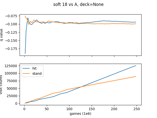
You can see that the only difference between the 2 results is the Soft 18 vs. a dealer Ace (1). For 1 deck, you should stand on soft 18 vs A, which matched Thorp’s 1966 book. For infinite decks, you should hit soft 18 vs A, which is the result that Sutton & Barto get in Reinforcement Learning (for an infinite deck).
As a quick check on our results, Thorp says that if you follow the “Basic Strategy” with no doubling or splitting, the “casino edge will be only about 2 percent.” We get a game value of -0.020, which seems like a good match.
Note that we have not included the ability to split pairs or double down, we will leave that as an exercise for the reader.
Just to see how close these two results are, here is a graph of the q value (average) for both deck types as we play the 250,000,000 games.