Review of The Perfect Bet

From 1993 to 2010, Joan Ginther won four jackpots in the Texas scratchcard lottery, totaling over $20 million.

Although Ginther has never commented on the reason for her multiple wins, some have speculated that her statistics PhD might have had something to do with it.

The Perfect Bet, by Adam Kucharski, 2016, Hachette Book Group.

Adam Kucharski, an assistant professor in mathematical modeling at the London School of Hygiene and Tropical Medicine, in his recent book, amuses and informs about the ways math and gambling have been connected throughout history.

In 1892, Karl Pearson decided to study the Le Monaco newpaper’s record of roulette outcomes to see if they were random.  As he studied the data, he found a number of anomalies.  Unfortunately for aspiring gamblers, it turns out that the data had been faked by reporters who were too lazy to record the actual numbers.

Kucharski outlines a number of cases where math did serve the gambler.

He talks about the MIT’s Ed Thorp, who basically invented blackjack card counting with his book Beat the dealer 1.

Did you know the Eudaemons built a roulette beating computer device 2? Hint: It has to do with physics, centripetal acceleration and friction.

He covers how Mohan Srivastava cracked an instant tic-tac-toe lottery game due to a design flaw. He details how teams, including one from MIT, beat the Massachusetts state lottery in the 2000s. See 3 for even more details on this one.

He talks about horse racing, including the use of modern techniques like machine learning, and how they have been applied to gambling. It’s not enough to just predict winners from results of previous races. It depends on which horses were running in those races and how they performed based on the groups they had been in previously, and so on.  It quickly become complicated.  But, as they say, if it were easy, everyone would be doing it.

From there, he moves on to soccer and sports betting.

He then take a few chapters to discuss the ins and outs of poker playing – both how computers have assisted players in improving their game, and how poker-bots have made a name for themselves in online poker rooms. There has also been an annual poker-bot competition at an academic artificial intelligence conference, where a team from the University of Alberta has dominated. Who knew?

While those looking for a handout of secrets to beating casino games will be somewhat disappointed, this book does provide some colorful background for those wanting to learn more about the ways math has been used in winning at gambling. It’s going to be up to you to figure it out.

Books mentioned here are available at Amazon:

The Perfect Bet, by Adam Kucharski
The Eudaemonic Pie, by Thomas Bass
Beat the Dealer, by Ed Thorp
How Not to be Wrong, by Jordan Ellenberg [My Review]


512 px Vdara Hotel

Starting a Fire With a Hotel

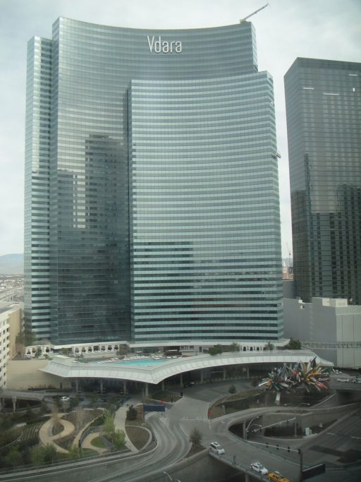
The Vdara hotel in Las Vegas gained some notoriety in 2010 when guests complained about getting severe burns from the pool deck area (see article). Note the curved facade and the pool and deck immediately below.  Image By Cygnusloop99 (Own work) [CC BY-SA 3.0 or GFDL], via Wikimedia Commons

Here is the view from Google maps. We will use this to get some measurements for the hotel:

We are going to build a simple simulation of the solar radiation reflection off the hotel mirrored facade. To this, we will need some things:

  1. The geometry of the hotel and pool deck area
  2. The orientation of the sun by time and date
  3. Calculations for reflection of the sun’s rays and their intersection with the pool deck.

Let’s take them in order.

Hotel Geometry

From a hotel floor plan, easily obtained on the web, we trace out the pool, pool deck, and facade surfaces.  Using the above satellite photo to get the scale properly, we then create 2 circular surfaces that closely match the facade geometry.  The radii of the 2 facades are 91.2m and 112.2m.  This is what the mathematical curves overlaid on the image look like. The axes are in meters and North is facing upward.  Notice that the curved surfaces have a very nice southern exposure.

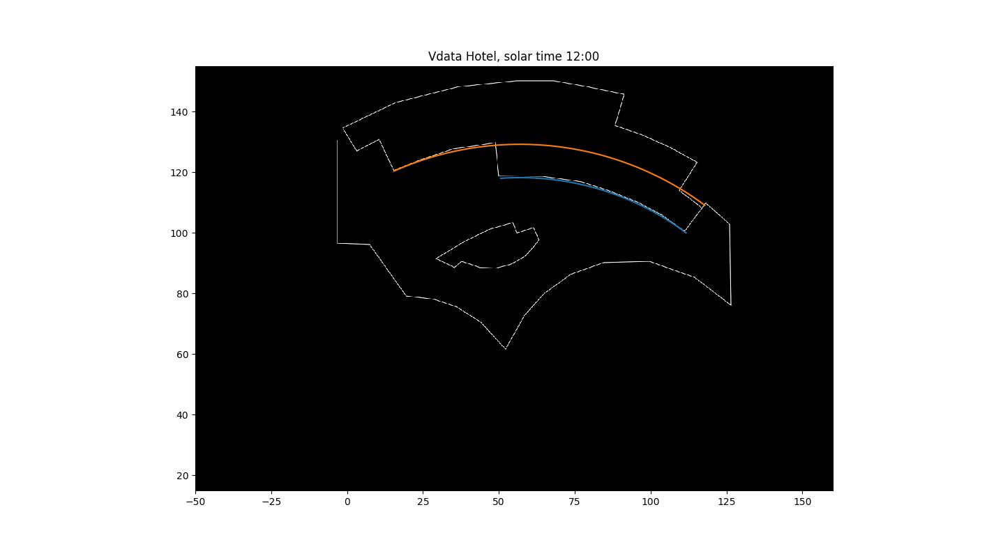
In this image, I have extended the second wall (orange) all the way in order to see how it fits on the floor plan. It is slightly above the floor plan at its right-most edge because there is a slight separation between the 3 semi-circular facades.
You can see the original floor plan here (rotated) Vdara Floor Plan.

Sun Orientation

The Wikipedia Sun Position article has a good introduction to the basic calculations.  We will review what we need here.  Basically, there are two coordinate systems that we will need.  The first is the ecliptic coordinate system, in which the sun and stars are (roughly speaking) constant.  Think of it as the stars’ coordinate system. In it, the ecliptic latitude is the angle from the plane of the Earth’s orbit around the Sun.  The ecliptic longitude of the Sun is zero when the Earth is at the vernal equinox.  So the ecliptic latitude of the Sun is 0, and the longitude depends on the day of the year, at least to the precision that we need for our solar convergence calculations.

The other coordinate system that we will need is the horizontal coordinate system.  This coordinate system is referenced to a viewer on a spot on the Earth, and has

  • Solar altitude: the angle above the horizon.  Its complementary angle is the Solar zenith.
  • Solar azimuth: the angle from the North, increasing clockwise towards the East.  Thus, 90 degrees is East and 180 degrees is South.

Rather than give all the equations for the calculations, which you can find on the Wikipedia page, I will give a Python function that will calculate the Sun’s position. The hour is the time before/after Solar Noon, which is when the Sun is at it’s highest point in the sky (close to Noon local time), and simpler to use here than trying to calculate from local time (which requires knowledge of time zones, etc.). Since we will be computing the Sun’s angle as it moves through the sky, the exact time is not important to us. If you want to check out when solar noon occurs, and compare the function below for accuracy, see NOAA Solar Calculations. For Las Vegas, the NOAA site matched this function within a few tenth’s of a degree.

def sun(hour, dt_noon=None):
  #compute sun at hour before/after solar noon on dt_noon, e.g. hour=-1 is 1 hour before solar noon
  if dt_noon is None:
    dt_noon=datetime.datetime(2017,8,24,hour=12,minute=0,second=0)
  #ecliptic coordinates
  n=(dt_noon - datetime.datetime(2000,1,1,hour=12)).days  #number of days since 1/1/2000
  L=(280.46+.9856474*n)/180*math.pi
  g=(357.528+.9856*n)/180*math.pi
  L=angle(L)  # make sure in 0-2*pi range
  g=angle(g)
  ecliptic_longitude=L+(1.915*math.sin(g)+0.020*math.sin(2*g))/180*math.pi
  ecliptic_latitude=0.0
  obliquity_of_ecliptic=23.4/180*math.pi

  hour_angle=(hour*15)/180*math.pi
  sun_declination=math.asin(math.sin(obliquity_of_ecliptic) * math.sin(ecliptic_longitude))

  solar_altitude=math.asin(math.sin(local_latitude)*math.sin(sun_declination)+
  math.cos(local_latitude)*math.cos(sun_declination)*math.cos(hour_angle))
  solar_zenith=math.pi/2-solar_altitude
  #solar_azimuth=math.pi-math.asin(-math.sin(hour_angle)*math.cos(sun_declination)/math.sin(solar_zenith))
  #solar_azimuth is measured by 0=north, 90 degrees=East, 180=South.
  #Note: problem when asin argument is around 1, because there are 2 solutions (like 85 and 95), so
  #we might get the wrong answer around sunrise/sunset.
  #This alternate version does not have the same problem, but we have to be careful about sign of h
  n1=math.sin(sun_declination)*math.cos(local_latitude) - 
  math.cos(hour_angle)*math.cos(sun_declination)*math.sin(local_latitude)
  d1=math.sin(solar_zenith)
  if (n1/d1) >= 1.0:
    solar_azimuth=0
  elif (n1/d1<-1.0):
    solar_azimuth=math.pi
  elif h<0:
    solar_azimuth=math.acos(n1/d1)
  else:
    solar_azimuth=2*math.pi-math.acos(n1/d1)
  return solar_altitude, solar_azimuth

Reflections and Intersections

The last piece we need are the calculations for reflections off surfaces.  If a light ray vector L impinges on a surface with unit normal N, it will be reflected with the same angle opposite the normal.  Looking at this figure:
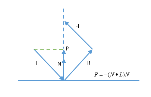
Ray Reflection

We can see that
\begin{align}
P=-(N \cdot L)N
\end{align}

because it is the projection of L onto the normal N.  Then we have

\begin{align}
R-L&=2P \\
R&=L-2(N \cdot L)N
\end{align}

Now that we have the reflected ray, we need to see how it intersects with the ground (or pool deck). For a plane described by a point \(p_0\) and normal \(n\) containing all points p such that:
\begin{align}
(p-p_0) \cdot n = 0
\end{align}

and a line described by a point \(l_0\) and a vector in the direction of the line \(l\) where the line is
\begin{align}
p=dl+l_0
\end{align}
points p for all real numbers l. If we solve these 2 equations for d, we get:
\begin{align}
d=\frac{(p_0-l_0) \cdot n}{l \cdot n}
\end{align}
which we can substitute back into the previous equation to get the intersection point \(p\).

Putting It All Together

Using Python and matplotlib, we can easily piece together a simulation of the intensity of the Sun’s rays.  To start, I tested the program with a simple flat facade in roughly the orientation of the first Vdara curved wall.
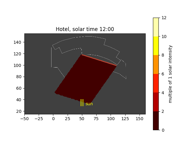
Flat hotel facade

The red line, at approximately -18 degrees, is the mirrors position on the floor plan.  The wall is 176m high, which is the height of the Vdara hotel.

The solar intensity is about 1.0 for the entire parallelogram image, which sort of what we would expect for a flat mirror.  It is not exactly 1 because the sun is not hitting the pool deck at exactly 90 degrees.  The 3 yellow lines represent the Sun’s azimuth.  Because this is solar 12:00 (solar noon), the azimuth is exactly 180 degrees.


Now, let us look at the results for the curved facade.

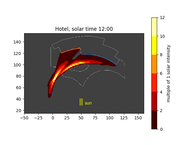
Solar noon at the hotel

Wow.  You can things are starting to heat up.  Believe it or not, the peak solar value is 15 in this plot.  A few things to be careful about:

  • I have not modeled the different heights of the 3 curved walls, nor the third wall that extends a little bit beyond the second wall
  • I have not modeled rays that have 2 or more reflections from their first intersection with the wall.  That is, some rays can hit the wall at an oblique enough angle to then hit the wall again.  In the figures to come, you can see that because some rays accumulate behind the wall, which would not happen in reality.
  • I have assumed that the walls are 100% reflective with no loss.  The architect did place some kind of plastic covering to reduce the reflection; how much has not been reported.  Also, with glass windows, some of the light passes through the window; how much is transmitted vs. reflected depend on the angle of incidence and the index of refraction of the glass.  A more accurate model would take this into account.

Now, placing several of these figures in an animation around solar noon, we can see how the hot spots move across the pool deck:

Solar convergence animation

Deep Trouble – Neural Networks Easily Fooled

Deep Neural Networks (DNNs) always leave me with a vague uneasy feeling in my stomach.  They seem to work well at image recognition tasks, yet we cannot really explain how they work.  How does the computer know that image is a fish, or a piano, or whatever?  Neural networks were originally modeled after how biological neurons were thought to work, although they quickly became a research area of their own without regard to biological operation.

Well, it turns out that DNNs don’t work at all like human brains.  A paper by Nguyen, et al 1 explores how easy it is to create images that look like nothing (white noise essentially) to the human brain, and yet are categorized with 99%+ certainty as a cheetah, peacock, etc. by DNNs that perform at human levels on standard image classification libraries.  Here a small sample of images from their paper:

The researchers created the false images through an evolutionary algorithm that seeks to modify existing images through mutation and combination in order to improve on a goal, in this case to find images that would score highly with a DNN classifier (“fooling images”).  They used a couple of methods, both of which worked.  The direct method, illustrated in the top two images, works by direct manipulation of the pixels in an image file.  The indirect method, illustrated in the bottom two images, works by using a series of formulas to generate the pixels; the formulas were then evolved.  The idea was to create images that looked more like images and less like random noise.  In both cases, the researchers found it easy to come up with images that fooled the DNN.

Their results also seemed robust.  They performed various trials with random starting points, they even added their fooling images to the training sets, so as to warn the DNN that these were incorrect.  Even after doing that, they were still able to find other fooling images that were misclassified by the new “improved” DNN.  They even repeated this process as many as 15 times, all to no avail.  The DNNs were still easily fooled.

As the authors point out, this ability of DNNs to be fooled has some serious implications for safety and security, for example in the area of self-driving cars.  For real world results, see the Self-driving car hack.

There is something going on here that we do not fully understand.  Researchers are starting to look into what features a DNN is really considering – which may help us to improve or alter the game for image recognition. Until then, pay attention to that pit in your stomach.

Notes:

  1. A. Nguyen, J Yosinkski, and J. Clune, Deep Neural Networks are Easily Fooled: High Confidence Predictions for Unrecognizable Images, Computer Vision and Pattern Recognition (CVPR ’15), IEEE, 2015

Bitcoin Network Hash Rates. Where are you, Bitcoin cash?

The Bitcoin blockchain just split in two.  What is Hash Power and where did it go?  With the split, people are discussing the terms “Hash Power” and trying to decide how many miners are mining each blockchain.  We will present the basic equations for working out these issues, and estimate the relative hash powers mining the 2 chains.

What is the Hash Rate?

Mining is the process by which the bitcoin blockchain is kept secure.  Briefly, the blockchain is a public ledger that everyone “agrees” on that contains the entire history of all bitcoin transaction since time began.  Miners do work (think mining gold) in order to add blocks to the blockchain, for which they get rewarded.  Bitcoin uses what’s called a Proof-of-Work system for mining, other methods used on other cryptos include Proof-of-Stake.

The basic work that the miner has to do is take a batch of current transactions, and find a number, called a nonce, so that the data (in a predetermined format) hashes to a number that is less than a target.

Let’s dissect these pieces one at a time:

  1. nonce: named because originally it was a “number used once”, but here it is just a number that the miner is free to pick.  Why the miner would want to pick different ones will be clear shortly.
  2. hash: A hash is a function that takes an arbitrary length piece of data and computes a digest, or shorter abbreviation for the data. Note: for the purists out there, we are just considering cryptographic hashes.  Bitcoin uses the hash SHA256, which is a particular hash that produces a 256 bit digest.  The idea of a good hash is that it is very hard to manipulate the data going into the hash to produce any particular hash – effectively it looks like a random number produced from the data (which is always the same for the same data).
  3. target: this is a 256 bit number.  Let’s call it T.  It gets calculated a special way on the Bitcoin network, as will be described later.

Now, to rehash things, so to speak:

To successfully add a block to the bitcoin blockchain, the miner must be the first person to find a nonce N, so that:
\[
\textrm{SHA256}(\textrm{SHA256}(\textrm{blockdata}, N)) < T
\]
where blockdata represents the transactions that the miner wants to include in the block. The nonce is in a certain place in that data, but here we call it out as a separate argument to make it clear that the results varies with N. Different miners might want to include different transactions for a variety of reasons, which we don’t need to go into here. Because of the properties of the SHA256 hash, this problem can only be solved (based on our current understanding of SHA256) by repeatedly trying different values of N until we find one that results in our target being hit. The miner has no idea which values of N are better than any others (because the hash is “random”), so they just try them in sequence, 0, 1, 2, 3, … until they find one that gives a hash value less than T. You might ask “why the double hash?”. Excellent question. No one knows for sure, but that’s just the way it is.

How long does it take for a miner to find an acceptable nonce?  Suppose that the miner can calculate H double-hashes per second.  Then, since the result of SHA256 is effectively a random number from 0 to \(2^{256}-1\), the probability of any given attempt satisfying the target is:
\[
prob=\frac{T}{2^{256}}
\]
and the expected time \(E(X)\)to find a new block would be
\[
E(X)=\frac{2^{256}}{T \cdot H}
\]

Difficulty

How is the target T calculated?  The target gets adjusted every 2016 blocks – the idea is that the average time for each block should be 10 minutes.  Thus, if there are so many miners that blocks are found much more frequently, say every 2 minutes, the target T would get adjusted (made smaller), so that the new block times become approximately 10 minutes.
Here are the details of the calculation. It uses something called the Difficulty (D), which is kind of the inverse of the T. That is, the higher difficulty, the lower the target T. You can find the current difficulty from a variety of websites, bitcoinwisdom.com has a nice graph of its history.

Remark: There is something called the packed difficulty (32 bits), which you may see. It is a floating-point representation of the difficulty which is shorter. For example, a packed difficulty 0x1d00ffff becomes:
\[
D_1=\text{0x00ffff} \cdot 2^{8 (\text{0x1d} – 3)}=\text{0xffff}\cdot 2^{208}=\text{0x00000000ffff0000000000000000000000000000000000000000000000000000}
\]
where there should be 52 0’s after the ffff. You can check my counting if you want.
This particular value of difficulty is called difficulty-1, \(D_1\).  It is the highest possible difficulty, and it used to compute the target from the current difficulty D.
\[
T=\frac{D_1}{D}
\]
If the current difficulty were \(D_1\), the target would be 1, and the SHA double hash would have to be 0. With a probability of that happening on each try of \(1/2^{256}\) or \(p=8.636 \cdot 10^{-78}\), that’s pretty hard! The expected number of hashes to find a block for a difficulty D is:
\[
\frac{2^{256}}{T}=\frac{D\cdot 2^{256}}{(2^{16}-1)2^{208}}\approx D\cdot2^{32}
\]
Let X be the time to find a block, we have the following relationships:
\begin{align}
T&=\frac{2^{256}}{D\cdot2^{32}}=\frac{2^{224}}{D}\\
\textrm{E}(X)&=\frac{2^{256}}{T \cdot H}=\frac{D \cdot 2^{32}}{H}
\end{align}
We can reverse the last equation to to estimate the number of hashes per second that a particular time to find a block represents:
\[
\text{hashpower (estimate)}=\frac{D\cdot 2^{32}}{X}
\]
Now, when we see the word “estimate”, we should be thinking “what is its variance?” The estimate here is zero-mean-error, but its variance is quite high. It turns out (I won’t prove it here) that if we expect \(\lambda\) blocks per second, then, for the time per block X:
\begin{align}
\textrm{E}(X)&=\frac{1}{\lambda} \\
\textrm{Var}(X)&=\frac{2}{\lambda^2}
\end{align}
Now, if we average block times over M blocks, the variance can be reduced per the usual formula:
\begin{align}
\textrm{Var}_M(X)&=\frac{2}{\lambda^2 \cdot M} \\
\textrm{std-dev}_M(X)&=\sqrt{\frac{2}{M}}\cdot \textrm{avg}(X)
\end{align}
For an example, the block times for bitcoin are generally around 10 minutes. If we average various numbers of past block times, we get the following standard deviations:

Number of Blocks Std Deviation of Average Block Time
6 5.77 min
10 4.47 min
20 3.16 min

Thus, we can see that even with looking at the last 20 blocks, we have a great uncertainty in the actual hash power that is operating to produce that block.  Let’s now look at the current block times for Bitcoin and Bitcoin cash and estimate the hash power operating on the chains.  Note that if mining hashpower is switching between Bitcoin and Bitcoin cash, it will take some time to determine that from the data – since we will want more than 20 blocks to average over.

Update 6 Aug 2017 10:47 AM EST:  blocktimes and difficulty dropped significantly (and BTC closer to expected average):

Bitcoin (BTC) Bitcoin Cash (BCC)
Avg Block Time (min) Std Dev Avg Block Time (min) Std Dev
Last 39 (BTC) 20 (BCC) blocks as of 10:47AM EST 6 Aug 2017 9.95 2.25 20.25 6.40
Difficulty 860 221 984 436 144 323 701 657
Estimated Hash Power (double-hash/sec) 6.19 * 10^18 5.1 * 10^17
Relative Hash Power (BTC=1.0) 1.0 .082


Note: this is current as of 5 Aug 2017 12:42 AM EST.  I hope to have a online updating version up later.

Bitcoin (BTC) Bitcoin Cash (BCC)
Avg Block Time (min) Std Dev Avg Block Time (min) Std Dev
Last 6 blocks 6.8 3.9 74.3 42.9
Last 20 blocks 6.0 1.9 76.0 24.0
Last 39 (BTC) 29 (BCC) blocks 5.7 1.5 55.6 12.6
Difficulty 860 221 984 436 225 505 642 691
Estimated Hash Power (double-hash/sec)  1.1 * 10^19  2.9 * 10^17
Relative Hash Power (BTC=1.0)  1.0 0.026

References

  1. Exponential Distribution
  2. Bitcoin Difficulty
  3. blockchair.com (for block times)
  4. A great detailed discussion of all aspects of bitcoin and other crytpocurrency concepts.
  5. Discussion geared for a less technical audience