Or, A Random Walk Down Bitcoin Avenue
A process follows a random walk if it has changes that are independent from one time interval to the next. A common question is “Does the price of X follow a random walk?” In particular, people are curious about the prices of stocks because they want to make money. Without getting too technical yet, if a price follows a random walk, you can’t make money trying to predict future prices. If you can show that it does not follow such a random walk, then it might be possible to make money at it. So, do stock prices follow a random walk?
| YES |
NO |
A Random Walk Down Wall Street
 
|
A Non-Random Walk Down Wall Street
  |
Bitcoin is a cryptocurrency, one of the better known ones, which uses something called Blockchain technology [look for future post on this topic]. There are several exchanges that allow one to buy and sell Bitcoins. So, a natural question would be “Do those prices follow a random walk?”
Let’s follow Prof. Andrew Lo’s excellent analysis from Chapter 2 of his book and see what conclusions we can draw about Bitcoin prices. Chapter 2 says that if the price change at period N+1 is independent of the price change at period N, then the variance over 2 periods should be twice the variance of changes over 1 period. Let \(X_n\) be the log-price of bitcoins for period \(n\).
Let’s derive the variance relationship. Let \(x, y\) be two random variables, and recall that the variance is the expected value of the squared deviation from the mean:
\[
var(x) \equiv E[ (x – \bar{x})^2 ]
\]
The variance of a sum of random variables
\begin{align}
var(x+y)=&E[ (x+y-\bar{x}-\bar{y})^2 ] \\
=&E[ (x-\bar{x})^2 + (y-\bar{y})^2 ] + 2 E[(x-\bar{x})(y-\bar{y})] \\
=&var(x) + var(y) + 2 cov(x,y)
\end{align}
Following Lo, let \(X_0,…,X_{nq} \) be the sequence of log-prices, and we define the variance ratio for period \(q\) as the variance at q steps divided by the variance at 1 step, divided again by q. This ratio should be 1.0 for all q if the steps are uncorrelated. Formally, letting \(\hat{\mu}\) be the mean increment, \(\bar{\sigma}_a^2\) be the variance estimate for 1 step, and \(\bar{\sigma}_c^2\) be the variance estimate for 1 step based on q-step differences, we have
\begin{gather}
\hat{\mu}=\frac{1}{nq} \sum_{k=1}^{nq}(X_k-X_{k-1})=\frac{1}{nq}(X_{nq}-X_0) \\
\bar{\sigma}_a^2= \frac{1}{nq-1} \sum_{k=1}^{nq}(X_k-X_{k-1}-\hat{\mu})^2 \\
\bar{\sigma}_c^2(q)= \frac{1}{m} \sum_{k=q}^{nq}(X_k-X_{k-q}-q\hat{\mu})^2 \\
m=q(nq-q+1)\left( 1 – \frac{q}{nq}\right)
\end{gather}
The results for running these calculations on Bitcoin prices from the BTC-e exchange from 2011, when trading started, to the present time (October 2016) is shown in table 1. Also shown in the table is the z-statistic \(z^*\) from Theorem 2.3 of Lo. This computes the significance of the variance ratio result. If the \(|z^*|\) is greater then 2, then the variance ratio result is significant at the .05 level, meaning that there is a only a 5% chance that the variance ratio differs from the null-hypothesis value of 1.
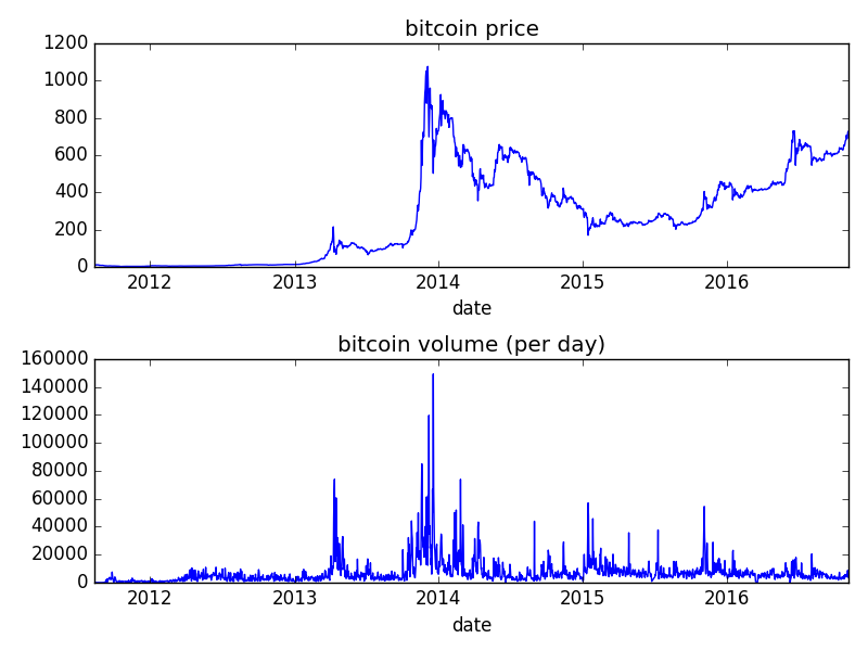
First, price and volume data for the time period of interest for the BTC-e exchange:
| Observation Period |
Years |
Num obs (nq) |
q=2 |
q=4 |
q=8 |
| 5 min |
2011-4 |
241,059 |
.729
(-3.39) |
.540
(-5.67) |
.411
(-7.04) |
| 2015-6 |
187,118 |
.853
(-17.04) |
.735
(-22.49) |
.670
(-21.80) |
| 1 hour |
2011-4 |
28,079 |
.791
(-6.47) |
.620
(-9.06) |
.568
(-8.20) |
| 2015-6 |
15,659 |
.940
(-2.40) |
.880
(-3.85) |
.855
(-3.46) |
| 1 day |
2011-4 |
1,234 |
.977
(-.27) |
.917
(-.82) |
.991
(-.07) |
| 2015-6 |
659 |
.983
(-.14) |
.869
(-.96) |
.862
(-.92) |
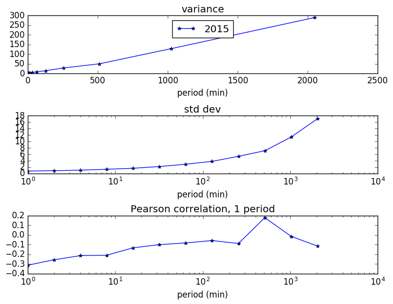
What conclusions that we can draw from this table?
- For 1 day periods, the variance ratio does not indicate any non-randomness.
- For shorter periods, there is significant non-randomness showing. In general, it looks like prices are negatively correlated with the prior period (because the variance ratio < 1.0). At 5 minute intervals, the correlation coefficient is approximately -0.15.
- The randomness has decreased since 2015.
- Note that from Lo’s book, (weekly) stock prices has variance rations > 1 (around 1.3), meaning that price changes were positively correlated. Note that the Bitcoin price changes are generally negatively correlated.
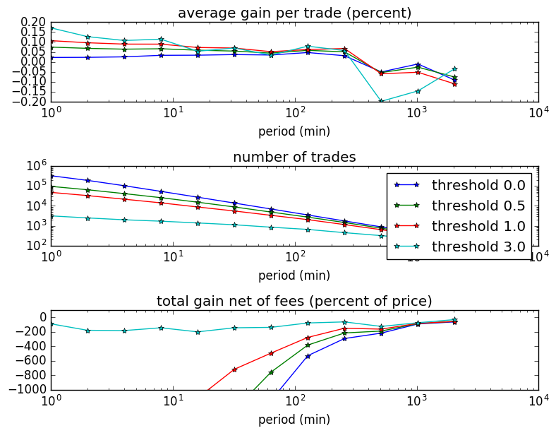
Our next post will look at whether you can profit from this non-randomness.