May 1, 2017February 15, 2022 by admin

PrimeGrid GPU Task Analysis

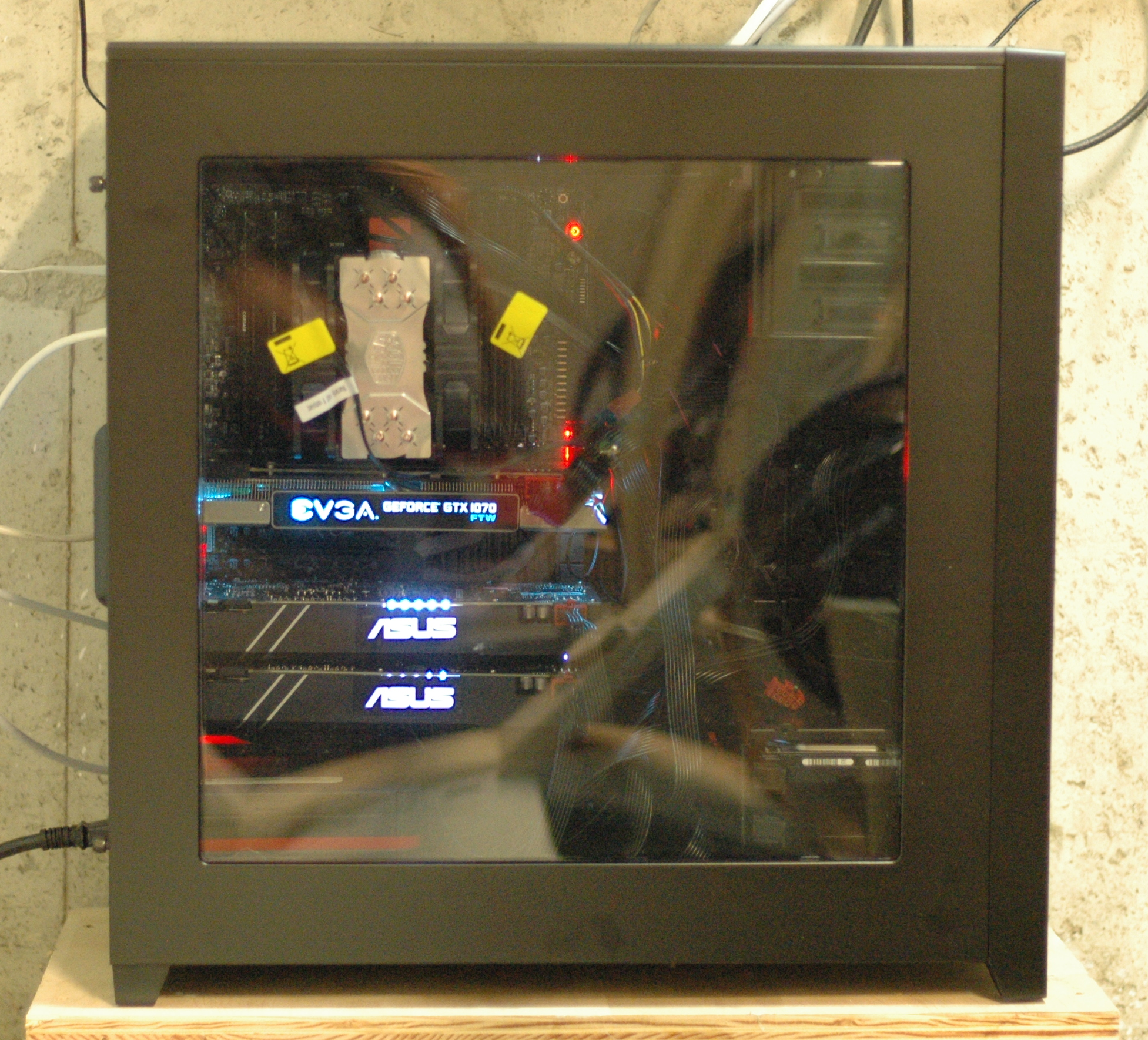
If you have a multi-GPU computer running on Primegrid.com, you might be wondering how to see how tasks are running across your GPUs. It turns out that the stderr log files can sometimes provide the GPU ID that was used to produce those results. I wrote a simple script that analyzes the run times by GPU; the script is located here:
https://gitlab.com/dgrunberg/primegrid-tasks

This is a snippet from the stderr output that it scans looking for gpu_device_num:

Unrecognized XML in parse_init_data_file: gpu_device_num
Skipping: 2
Skipping: /gpu_device_num
Unrecognized XML in parse_init_data_file: gpu_opencl_dev_index
Skipping: 2
Skipping: /gpu_opencl_dev_index
Unrecognized XML in parse_init_data_file: gpu_usage
Skipping: 1.000000

Sample output:

Processing tasks for hostid 820440
====================================


                              run-avg  run-std  run-count  credit-avg  credit-cnt  credit_per_s
date       gpu  task                                                                           
2017-05-01 0    pps_sr2sieve    404.7     2.21         91      3371.0          43         8.330
           1    pps_sr2sieve    424.8     3.42         86      3371.0          39         7.936
           2    pps_sr2sieve    387.1     2.51         93      3371.0          38         8.709
           none llrPPS         1768.6   184.86         16       119.9          10         0.068
                llrSGS          652.5    14.17        103        39.9          46         0.061

                   run-avg  run-std  run-count  credit-avg  credit-cnt  credit_per_s
gpu  task                                                                           
0    pps_sr2sieve    404.7     2.21         91      3371.0          43         8.330
1    pps_sr2sieve    424.8     3.42         86      3371.0          39         7.936
2    pps_sr2sieve    387.1     2.51         93      3371.0          38         8.709
none llrPPS         1768.6   184.86         16       119.9          10         0.068
     llrSGS          652.5    14.17        103        39.9          46         0.061

Tasks: Processed:400, Completed:389 New files requested:37 Total time: 20.41 sec

April 10, 2017April 10, 2017 by admin

Installing BOINC on Multi GPU Computer

Follow @solverworld Tweet this

Computer GPUs lit up

Already built a multi-GPU computer? No? See How to Build a Multi-GPU Computer here.

OK, we have our multiple GPU system wired up and it seems to boot OK into the BIOS. The BIOS shows our 3 GPUs installed in the proper slots and we like the speeds (Gen 3) of PCIe that are chosen.

Let’s install Linux. I choose Debian – I am familiar with it, and more importantly, I got it to work with BOINC. Here is that procedure:

Create a netinst DVD or CD for Debian Stretch. I found that the latest stable version (Jessie) did not have the correct packages to get BOINC running. I used RC2, but RC3 is available now, and should work as well. Ddownload the .iso file you need (probably the amd64 package) to your computer, then use an ISO writing program to write that to a DVD/CD. On a Windows machine, I used ImgBurn, but you can use any program you like.
Boot the multi-GPU computer with this DVD. If it does not boot from the DVD drive, you will need to go into the BIOS and set up the boot order so that the DVD is first or at least tried after the HDD fails.
Follow the prompts to install Debian. There are plenty of guides on the Internet to help you, but it is pretty straightforward. You can take defaults for just about everything. I did NOT install the desktop environment because I only plan on ssh’ing into the computer and did not want to have X software installed/running. Do choose ssh server and standard system utilities. NOTE: you will need an Internet connection, preferably hardwired, to install Debian, so plug in an Ethernet cable to your Internet connection before you start.
Install sudo so you can become root as needed – first log in as root, then
```
apt-get install sudo
usermod -aG sudo <your-user-name>
```
Add contrib and non-free to your /etc/apt/sources.lst file as some of the nvidia driver files are in those categories. You should have a line in the sources.lst file that looks like:
```
deb http://ftp.us.debian.org/debian/ stretch main non-free contrib
```
Update your database:
```
sudo apt-get update
```
To be able to ssh into this machine without a password, add your public key which you have copied to this machine already, to the list of authorized keys. Note that you could transfer the key with a USB key if you don’t want to copy over the network:
```
sudo mount /dev/sdb1 /media/usb    # your devices may differ
cat /media/usb/id_rsa.pub >> ~/.ssh/authorized_keys
```
Now install the BOINC software and related drivers. You might want to install them sequentially to make debugging simpler in case something goes wrong. I got nvidia-driver version 375.26-2.
```
sudo apt-get install nvidia-driver boinc-client-opencl boinc-client-nvidia-cuda boinc
```
Make sure the BOINC client autostarts on boot up – check your /etc/init.d/ directory for a boinc-client script. Now, a small adjustment is necessary to make sure the GPUs are detected at startup – there is a race condition with drivers, so edit the boinc-client script (as root) and add a sleep 2.0 line so that the start() function in the file looks like:
```
start()
{
 log_begin_msg "Starting $DESC: $NAME me"
 sleep 2.0    #<== ADD THIS LINE
 if is_running; then
   log_progress_msg "already running"
 else
   if
```
Now, you should be able to reboot the computer and see something like the following from ps -ef:
```
#ps -ef |grep boinc
dan      614 24444 0 17:17 pts/0 00:00:00 grep boinc
boinc    623 1     0 Mar30 ?     00:00:00 /bin/sh -c /usr/bin/boinc --dir /var/lib/boinc-client >/var/log/boinc.log 2>/var/log/boincerr.log
boinc    641 623   0 Mar30 ?     00:30:05 /usr/bin/boinc --dir /var/lib/boinc-client
```
If you can’t see boinc, running you will need to do some debugging. Check out /var/log/boinc.log and you can see the startup messages. If everything is going well, you will see the GPUs being detected and indicating how many are usable (hopefully the number you installed, in this case 3). Some debug steps are: (i) try nvidia-smi to see if the Nvidia drivers can see your GPUs, and (ii) set the BOINC logging flags – possibly <coproc_debug> in BOINC Configuration.
A couple more things and we are almost done. To enable remote management of the BOINC server software, add/edit the following files in /var/lib/boinc_client:
```
echo <remote-access-password> > gui_rpc_auth.cfg
echo <your-remote-access-IP-address> > remote_hosts.cfg
```
Now you should be able to connect to the server through the boincmgr program, using the password you set above. You can install BOINC on a windows or linux machine fairly easily, which will give you access to the manager program. Of course, if you want to keep your GPU machine in a place where you can access it via keyboard and monitor, you could just run the boincmgr locally. Note that it will not run unless you install a Desktop environment, since it needs X-client running.
From the manager program, you can select a project from the available ones on BOINC such as SETI, primegrid, etc. You will have to provided credentials to get you started, which you get by creating an account on the appropriate projects website (e.g. primegrid.com). For Primegrid, you can control which tasks your computer works on through configuring things on the primegrid website. Note that only certain tasks can take advantage of the Nvidia-cuda GPUs, so make sure you select at least 1 subproject that does that. Other tasks can be run on the CPU directly, but make sure not to fully load your CPU with tasks, as that will tend to slow down the servicing of the GPUs.
If your computer will have any exposure to the outside world (including your home WiFi), you should be careful to secure it properly. At a minimum, you will want to disable root logins, all unnecessary processes and open ports.
Join the SolverWorld team on PrimeGrid and add your computing power to the team. I will announce your contributions (if you want) on separate page in the future.
Happy computing!

February 9, 2017February 15, 2022 by admin

Trading Stochastic Difference Equations

Follow @solverworld Tweet this

If you haven’t read Part 1, do that first.
$\newcommand{\Var}{\mathrm{Var}}$
$\newcommand{\Cov}{\mathrm{Cov}}$
$\newcommand{\Expect}{{\rm I\kern-.3em E}}$
$\newcommand{\me}{\mathrm{e}}$
For a quick review, recall that our system looks like:
\begin{align}
x_{n+1}&=ax_n+w_n \\
w_n &\sim N(0, \sigma^2) \\
|a| & < 1. \\
\end{align}
Next, let’s define a time constant, $\tau$, that gives us an idea of how the noise term, $w_n$, is filtered. Time constants are generally the time it takes to reach $1/\me$ of a steady-state value, so:
\begin{align}
&\frac{1}{\me}=a^\tau \\
&-1=\tau \ln a\\
&\tau=\frac{-1}{\ln a}\\
\text{or}\\
&a=\me^{-1/ \tau}
\end{align}

Now, our goal is to understand how we could trade (profitably) such a stochastic system. What does this mean? We might want to try something like, “buy low, sell high.” Like
\begin{align}
x_n \leq T_1&\Rightarrow \text{buy}\\
x_n \geq T_2&\Rightarrow \text{sell}
\end{align}
Our profit on each round-trip trade would be $T_2-T_1$. Hopefully, we choose $T_2 > T_1$.

Thresholds

Since our system is linear, scaling the input ($w_n$), scales the output. Thus, if we set thresholds as a multiple of $\sigma$ we do not have to explore different noise powers. Put another way, if we fix, say, $\Var(x)\equiv 1$, then we can experiment with different thresholds, and the results will hold for those thresholds as a multiple of $\Var(x)$.

Time Durations

Similarly, if we are counting events (trades) over time, we want to be able to scale everything to a useful value.
Consider (from Part 1):

\begin{align}
\Var(x_k-x_0)&=2 \sigma^2 \frac{1-a^k}{1-a^2} \\
&=2\Var(x)(1-a^k)\\
&=2\Var(x)(1-\me^{-k/\tau})
\end{align}
We can see that the variance of increments depends on the number of time constants that we go out. So, if we count trades per time constant interval, we will have standardized our results. Note: The astute reader should note that this is not a proof (not even close), but we will leave that for later. This is more of a “seems plausible.”

Some Simulations

Let’s perform a few tests to get started. We will pick an $a$ corresponding to $\tau$ of [300, 600, 1200] time steps (think seconds), and then fix $\sigma$ to make $\Var(x)\equiv 1$. Then we will perform Monte Carlo simulations over enough time steps to get statistically significant results.

Here are the results.

There are 2 types of trading algorithms simulated here:

-t/+t: buy when x<-t and sell when x>+t, count action as 0.5 trades
-2t/0/+2t: buy when x<-2t and sell when x>0; plus sell when x>2t and buy when x<0

Each of these has a 2t profit per round trip trade, but the second option occurs more often for smaller thresholds. For larger thresholds, the rapid Gaussian falloff causes there to be fewer trades.

Note you can see that the three different time constant (TC) values have lines very close to each other, justifying our supposition that events per TC are the relevant experimental parameter. This means we can do our simulations for a single TC, rather than a whole series.

If we multiple the number of trades by the profit per trade, we get the following result. Of course, this ignores commissions, which would drag down the profits more on the lower thresholds (more trades).

The simulations used 200,000 time steps, and the following parameters.

time constant (steps)	a	std dev of w	std dev of x
300	.99667	.082	1.031
600	.99833	.058	1.029
1200	.99917	.041	1.005

November 14, 2016February 15, 2022 by admin

Do Bitcoin Prices Walk Randomly?

Follow @solverworld Tweet this

Or, A Random Walk Down Bitcoin Avenue

A process follows a random walk if it has changes that are independent from one time interval to the next. A common question is “Does the price of X follow a random walk?” In particular, people are curious about the prices of stocks because they want to make money. Without getting too technical yet, if a price follows a random walk, you can’t make money trying to predict future prices. If you can show that it does not follow such a random walk, then it might be possible to make money at it. So, do stock prices follow a random walk?

YES	NO
A Random Walk Down Wall Street ¹	A Non-Random Walk Down Wall Street ²

Bitcoin is a cryptocurrency, one of the better known ones, which uses something called Blockchain technology [look for future post on this topic]. There are several exchanges that allow one to buy and sell Bitcoins. So, a natural question would be “Do those prices follow a random walk?”

Let’s follow Prof. Andrew Lo’s excellent analysis from Chapter 2 of his book and see what conclusions we can draw about Bitcoin prices. Chapter 2 says that if the price change at period N+1 is independent of the price change at period N, then the variance over 2 periods should be twice the variance of changes over 1 period. Let $X_n$ be the log-price of bitcoins for period $n$.

Let’s derive the variance relationship. Let $x, y$ be two random variables, and recall that the variance is the expected value of the squared deviation from the mean:

\[
var(x) \equiv E[ (x – \bar{x})^2 ]
\]

The variance of a sum of random variables

\begin{align}
var(x+y)=&E[ (x+y-\bar{x}-\bar{y})^2 ] \\
=&E[ (x-\bar{x})^2 + (y-\bar{y})^2 ] + 2 E[(x-\bar{x})(y-\bar{y})] \\
=&var(x) + var(y) + 2 cov(x,y)
\end{align}

Following Lo, let $X_0,…,X_{nq} $ be the sequence of log-prices, and we define the variance ratio for period $q$ as the variance at q steps divided by the variance at 1 step, divided again by q. This ratio should be 1.0 for all q if the steps are uncorrelated. Formally, letting $\hat{\mu}$ be the mean increment, $\bar{\sigma}_a^2$ be the variance estimate for 1 step, and $\bar{\sigma}_c^2$ be the variance estimate for 1 step based on q-step differences, we have

\begin{gather}
\hat{\mu}=\frac{1}{nq} \sum_{k=1}^{nq}(X_k-X_{k-1})=\frac{1}{nq}(X_{nq}-X_0) \\
\bar{\sigma}_a^2= \frac{1}{nq-1} \sum_{k=1}^{nq}(X_k-X_{k-1}-\hat{\mu})^2 \\
\bar{\sigma}_c^2(q)= \frac{1}{m} \sum_{k=q}^{nq}(X_k-X_{k-q}-q\hat{\mu})^2 \\
m=q(nq-q+1)\left( 1 – \frac{q}{nq}\right)
\end{gather}

The results for running these calculations on Bitcoin prices from the BTC-e exchange from 2011, when trading started, to the present time (October 2016) is shown in table 1. Also shown in the table is the z-statistic $z^*$ from Theorem 2.3 of Lo. This computes the significance of the variance ratio result. If the $|z^*|$ is greater then 2, then the variance ratio result is significant at the .05 level, meaning that there is a only a 5% chance that the variance ratio differs from the null-hypothesis value of 1.

First, price and volume data for the time period of interest for the BTC-e exchange:

Observation Period	Years	Num obs (nq)	q=2	q=4	q=8
5 min	2011-4	241,059	.729 (-3.39)	.540 (-5.67)	.411 (-7.04)
5 min	2015-6	187,118	.853 (-17.04)	.735 (-22.49)	.670 (-21.80)
1 hour	2011-4	28,079	.791 (-6.47)	.620 (-9.06)	.568 (-8.20)
1 hour	2015-6	15,659	.940 (-2.40)	.880 (-3.85)	.855 (-3.46)
1 day	2011-4	1,234	.977 (-.27)	.917 (-.82)	.991 (-.07)
1 day	2015-6	659	.983 (-.14)	.869 (-.96)	.862 (-.92)

What conclusions that we can draw from this table?

For 1 day periods, the variance ratio does not indicate any non-randomness.
For shorter periods, there is significant non-randomness showing. In general, it looks like prices are negatively correlated with the prior period (because the variance ratio < 1.0). At 5 minute intervals, the correlation coefficient is approximately -0.15.
The randomness has decreased since 2015.
Note that from Lo’s book, (weekly) stock prices has variance rations > 1 (around 1.3), meaning that price changes were positively correlated. Note that the Bitcoin price changes are generally negatively correlated.

Our next post will look at whether you can profit from this non-randomness.

Notes:

A Random Walk Down Wall Street, 11th ed., Burton G. Malkiel 2016, 1st ed 1973. ↩
A Non-Random Walk Down Wall Street, Andrew W. Lo & A. Craig MacKinlay, 2002 ↩

Business

Blackjack Strategy – A Monte Carlo Method

DIY Hand Sanitizer – Methanol is Deadly

An Investor’s View of ICOs

Lending Rates for Bitcoin and USD on Cryptoexchanges